11 Access Census Data with the tidycensus Package

If you’ve ever worked with data from the United States Census Bureau, you know what a hassle it can be. You’ve got to go to the Census Bureau website, find the data you need, download it, and then analyze it in your tool of choice. Working with Census Bureau data in this way involves a lot of pointing and clicking, and gets very tedious over time.

This tedium is what drove Texas Christian University geographer Kyle Walker to develop a package to automate the process of bringing Census Bureau data into R. Walker had previously created a package called tigris (introduced in Chapter 4) to automatically bring in shape files from the Census Bureau. As he told me, “I was using tigris pretty heavily in my own work to bring in the spatial data, but I didn’t have a seamless way to get the demographic data as well.” Drawing on his experience developing tigris, Walker, along with co-author Matt Herman (yes, he of the Westchester COVID-19 website discussed in Chapter 9), would develop the tidycensus package, which allows R users to bring in data directly from various Census Bureau datasets. With tidycensus, a user can write just a few lines of code and get data on, say, the median income in all 3,000 plus counties in the United States.

In this chapter, we’ll learn how the tidycensus package works. We’ll do this using examples from two datasets that tidyverse makes it possible to work with: the every-ten-year (decennial) Census and the American Community Survey. We’ll also show how we can use the data from these two sources for additional analysis and to make maps by accessing geospatial and demographic data simultaneously. While this chapter focuses on data from the United States Census Bureau, the conclusion lists other R packages that access analogous data from other countries. And finally, the conclusion highlights some of the reasons why using a package like tidycensus can improve your workflow.

Using tidycensus

The tidycensus package is available on CRAN so you can install it as you would most packages using install.packages("tidycensus"). In order to use tidycensus you must also get an API (application programming interface) key from the Census Bureau. This key, which is free, can be obtained by going to https://api.census.gov/data/key_signup.html and entering your details. Once you receive your API key by email, you need to put it in a place where tidycensus can find it. The census_api_key() function does this for you. Your best bet, after loading the tidycensus package, is to run the function as follows (replacing 123456789 with your actual API key):

library(tidycensus)

census_api_key("123456789", install = TRUE)

The install = TRUE argument will save your API key in your .Renviron file (a file designed to keep confidential information like API keys). The tidycensus will look for your API key there in the future so that you don’t have to enter it every time you want to use the package.

Having obtained and saved our API key, we’re now ready to use tidycensus to access data. The Census Bureau puts out many datasets, several of which can be accessed using tidycensus. The most common datasets to access with tidycensus are the decennial Census and the American Community Survey (other datasets that can be accessed are discussed in Chapter 2 of Kyle Walker’s book Analyzing US Census Data: Methods, Maps, and Models in R).

Working with Decennial Census Data

We’ll start out by accessing data from the 2020 Census on the Asian population in each state. To do this, we use the get_decennial() function with three arguments:

get_decennial(geography = "state", 
              variables = "P1_006N",
              year = 2020)

The arguments we’re using here are:

• geography, which tells get_decennial() to access data at the state level. There are many other geographies, including county, census tract, and more.
• variables is where we choose the variable or variables we want to access. I know that P2_002N is the variable name for the total Asian, but below I’ll demonstrate how to identify other variables you may want to use.
• year is where we select the year from which we want to access data. We’re using data from the 2020 Census.

Running this code returns the following:

#> # A tibble: 52 × 4
#>    GEOID NAME                 variable   value
#>    <chr> <chr>                <chr>      <dbl>
#>  1 42    Pennsylvania         P1_006N   510501
#>  2 06    California           P1_006N  6085947
#>  3 54    West Virginia        P1_006N    15109
#>  4 49    Utah                 P1_006N    80438
#>  5 36    New York             P1_006N  1933127
#>  6 11    District of Columbia P1_006N    33545
#>  7 02    Alaska               P1_006N    44032
#>  8 12    Florida              P1_006N   643682
#>  9 45    South Carolina       P1_006N    90466
#> 10 38    North Dakota         P1_006N    13213
#> # … with 42 more rows

The resulting data frame has four variables:

• GEOID is the geographic identifier given by the Census Bureau for the state. Each state has a geographic identifier, as do all counties, census tracts, and all other geographies.
• NAME is the name of each state.
• variable is the name of the variable we passed to the get_decennial() function.
• value is the numeric value for the state and variable in each row. In our case, it represents the total Asian population in each state.

Let’s say we want to calculate the Asian population as a percentage of all people in each state. To do that, we’d need both the Asian population as well as the total population. How would we do this?

Identifying Variables

First, we’d need to know the variable names. I looked up the variable name for Asian population (P1_006N) without showing you how I did it. Let’s backtrack so I can show you how to identify variable names. The tidycensus package has a function called load_variables() that shows us all of the variables from the decennial Census. If we run it with the argument year set to 2020 and dataset set to “pl” (pl refers to public law 94-171, which requires the Census to produce so-called redistricting summary data files every ten years).

load_variables(year = 2020, 
               dataset = "pl")

Running this code returns the name, label (description), and concept (category) of all variables available to us. Looking at this, we can see variable P1_006N (it’s cut off here, but in RStudio you’d see the full description). We can also see that variable P1_001N gives us the total population.

#> # A tibble: 301 × 3
#>    name    label                                     concept
#>    <chr>   <chr>                                     <chr>  
#>  1 H1_001N " !!Total:"                               OCCUPA…
#>  2 H1_002N " !!Total:!!Occupied"                     OCCUPA…
#>  3 H1_003N " !!Total:!!Vacant"                       OCCUPA…
#>  4 P1_001N " !!Total:"                               RACE   
#>  5 P1_002N " !!Total:!!Population of one race:"      RACE   
#>  6 P1_003N " !!Total:!!Population of one race:!!Whi… RACE   
#>  7 P1_004N " !!Total:!!Population of one race:!!Bla… RACE   
#>  8 P1_005N " !!Total:!!Population of one race:!!Ame… RACE   
#>  9 P1_006N " !!Total:!!Population of one race:!!Asi… RACE   
#> 10 P1_007N " !!Total:!!Population of one race:!!Nat… RACE   
#> # … with 291 more rows

Using Multiple Variables

Now that we know which variables we need, we can use the get_decennial() function again. We used just one variable above, but we can run our code again with two variables.

get_decennial(geography = "state", 
              variables = c("P1_001N", "P1_006N"),
              year = 2020) %>% 
  arrange(NAME)

I’ve added arrange(NAME) after get_decennial() so that the results are sorted by state name, allowing us to see that we have both variables for each state.

#> # A tibble: 104 × 4
#>    GEOID NAME       variable    value
#>    <chr> <chr>      <chr>       <dbl>
#>  1 01    Alabama    P1_001N   5024279
#>  2 01    Alabama    P1_006N     76660
#>  3 02    Alaska     P1_001N    733391
#>  4 02    Alaska     P1_006N     44032
#>  5 04    Arizona    P1_001N   7151502
#>  6 04    Arizona    P1_006N    257430
#>  7 05    Arkansas   P1_001N   3011524
#>  8 05    Arkansas   P1_006N     51839
#>  9 06    California P1_001N  39538223
#> 10 06    California P1_006N   6085947
#> # … with 94 more rows

Giving Variables Better Names

I often have trouble remembering what variable names like P1_001N and P1_006N mean. Fortunately, we can adjust our code in get_decennial() to give our variables more meaningful names using the following syntax:

get_decennial(geography = "state", 
              variables = c(total_population = "P1_001N", 
                            asian_population = "P1_006N"),
              year = 2020) %>% 
  arrange(NAME)

When we run this code, it is now much easier to remember which variables we are working with.

#> # A tibble: 104 × 4
#>    GEOID NAME       variable            value
#>    <chr> <chr>      <chr>               <dbl>
#>  1 01    Alabama    total_population  5024279
#>  2 01    Alabama    asian_population    76660
#>  3 02    Alaska     total_population   733391
#>  4 02    Alaska     asian_population    44032
#>  5 04    Arizona    total_population  7151502
#>  6 04    Arizona    asian_population   257430
#>  7 05    Arkansas   total_population  3011524
#>  8 05    Arkansas   asian_population    51839
#>  9 06    California total_population 39538223
#> 10 06    California asian_population  6085947
#> # … with 94 more rows

Instead of “P1_001N” and “P1_006N”, we have “total_population” and “asian_population.” Much better!

Analyzing Census Data

Let’s now return to what started us down this path: calculating the Asian population in each state as a percentage of the total. To do this, we use the code from above and add a few things to it:

1. We use group_by(NAME) to create one group for each state because we want to calculate the Asian population percentage in each state.
2. We use mutate(pct = value / sum(value)) to calculate the percentage. This line takes the value in each row and divides it by the total_population and asian_population rows for each state.
3. We use ungroup() to remove the state-level grouping.
4. We use filter(variable == "asian_population") to only show the Asian population percentage.

get_decennial(geography = "state", 
              variables = c(total_population = "P1_001N", 
                            asian_population = "P1_006N"),
              year = 2020) %>% 
  arrange(NAME) %>% 
  group_by(NAME) %>% 
  mutate(pct = value / sum(value)) %>% 
  ungroup() %>% 
  filter(variable == "asian_population")

When we run this code, we see the Asian population and the Asian population as a percentage of the total population in each state.

#> # A tibble: 52 × 5
#>    GEOID NAME                 variable        value      pct
#>    <chr> <chr>                <chr>           <dbl>    <dbl>
#>  1 01    Alabama              asian_popula…   76660 0.015029
#>  2 02    Alaska               asian_popula…   44032 0.056638
#>  3 04    Arizona              asian_popula…  257430 0.034746
#>  4 05    Arkansas             asian_popula…   51839 0.016922
#>  5 06    California           asian_popula… 6085947 0.13339 
#>  6 08    Colorado             asian_popula…  199827 0.033452
#>  7 09    Connecticut          asian_popula…  172455 0.045642
#>  8 10    Delaware             asian_popula…   42699 0.041349
#>  9 11    District of Columbia asian_popula…   33545 0.046391
#> 10 12    Florida              asian_popula…  643682 0.029018
#> # … with 42 more rows

Using a Summary Variable

Kyle Walker knew that calculating summaries like this would be a common use case for tidycensus. So, to simplify things, he gives us the summary_var argument that we can use within get_decennial(). Instead of putting “P1_001N” (total population) in the variables argument, we can instead use it with the summary_var argument as follows.

get_decennial(geography = "state", 
              variables = c(asian_population = "P1_006N"),
              summary_var = "P1_001N",
              year = 2020) %>% 
  arrange(NAME)

This returns a nearly identical data frame to what we got above, except that the total population is now a separate variable, rather than additional rows for each state.

#> # A tibble: 52 × 5
#>    GEOID NAME                 variable        value summar…¹
#>    <chr> <chr>                <chr>           <dbl>    <dbl>
#>  1 01    Alabama              asian_popula…   76660  5024279
#>  2 02    Alaska               asian_popula…   44032   733391
#>  3 04    Arizona              asian_popula…  257430  7151502
#>  4 05    Arkansas             asian_popula…   51839  3011524
#>  5 06    California           asian_popula… 6085947 39538223
#>  6 08    Colorado             asian_popula…  199827  5773714
#>  7 09    Connecticut          asian_popula…  172455  3605944
#>  8 10    Delaware             asian_popula…   42699   989948
#>  9 11    District of Columbia asian_popula…   33545   689545
#> 10 12    Florida              asian_popula…  643682 21538187
#> # … with 42 more rows, and abbreviated variable name
#> #   ¹​summary_value

With our data in this new format, we can calculate the Asian population as a percentage of the whole by dividing the value variable by the summary_value variable.

get_decennial(geography = "state", 
              variables = c(asian_population = "P1_006N"),
              summary_var = "P1_001N",
              year = 2020) %>% 
  arrange(NAME) %>% 
  mutate(pct = value / summary_value)

The resulting output is nearly identical.

#> # A tibble: 52 × 6
#>    GEOID NAME              varia…¹   value summar…²      pct
#>    <chr> <chr>             <chr>     <dbl>    <dbl>    <dbl>
#>  1 01    Alabama           asian_…   76660  5024279 0.015258
#>  2 02    Alaska            asian_…   44032   733391 0.060039
#>  3 04    Arizona           asian_…  257430  7151502 0.035997
#>  4 05    Arkansas          asian_…   51839  3011524 0.017214
#>  5 06    California        asian_… 6085947 39538223 0.15393 
#>  6 08    Colorado          asian_…  199827  5773714 0.034610
#>  7 09    Connecticut       asian_…  172455  3605944 0.047825
#>  8 10    Delaware          asian_…   42699   989948 0.043133
#>  9 11    District of Colu… asian_…   33545   689545 0.048648
#> 10 12    Florida           asian_…  643682 21538187 0.029886
#> # … with 42 more rows, and abbreviated variable names
#> #   ¹​variable, ²​summary_value

How you choose to calculate summary statistics is up to you. The good thing is that tidycensus makes it easy to do either way!

Working with American Community Survey Data

Let’s switch now to accessing data from the American Community Survey (ACS). This survey, which is conducted every year, differs from the decennial Census in two major ways:

1. It is given to a sample of people rather than the entire population.
2. It includes a wider range of questions.

Despite these differences, accessing data from the ACS is nearly identical to how we access Census data. Instead of get_decennial(), we use the function get_acs(), but the arguments are the same. Here I’ve identified a variable I’m interested in (B01002_001, which shows median age) and am using it to get the data for each state.

get_acs(geography = "state",
        variables = "B01002_001",
        year = 2020)

Here’s what the output looks like:

#> # A tibble: 52 × 5
#>    GEOID NAME                 variable   estimate   moe
#>    <chr> <chr>                <chr>         <dbl> <dbl>
#>  1 01    Alabama              B01002_001     39.2   0.1
#>  2 02    Alaska               B01002_001     34.6   0.2
#>  3 04    Arizona              B01002_001     37.9   0.2
#>  4 05    Arkansas             B01002_001     38.3   0.2
#>  5 06    California           B01002_001     36.7   0.1
#>  6 08    Colorado             B01002_001     36.9   0.1
#>  7 09    Connecticut          B01002_001     41.1   0.2
#>  8 10    Delaware             B01002_001     41     0.2
#>  9 11    District of Columbia B01002_001     34.1   0.1
#> 10 12    Florida              B01002_001     42.2   0.2
#> # … with 42 more rows

There are two differences we can see in the get_acs() output compared to that from get_decennial():

1. The value column in get_decennial() is called estimate with get_acs().
2. We have an additional column called moe for margin of error.

Both of these changes are because the ACS is given to a sample of the population. As a result, we don’t have precise values, but rather estimates, which are extrapolations from the sample to the population as a whole. And with an estimate comes a margin of error. In our state-level data, the margins of error are relatively low, but if you get data from smaller geographies, they tend to be higher. In cases where your margins of error are high relative to your estimates, you should interpret results with caution, as there is greater uncertainty about how well the data represents the population as a whole.

Using ACS Data to Make Charts

As we saw with Census data on the Asian population in the United States, once you access data using the tidycensus package, you can do whatever else you want with it. We calculated the Asian population as a percentage of the total above. Here we could take the data on median age and pipe it into ggplot in order to create a bar chart.

get_acs(geography = "state",
        variables = "B01002_001",
        year = 2020) %>% 
  ggplot(aes(x = estimate,
             y = NAME)) +
  geom_col()

Figure 11.1 shows our bar chart.

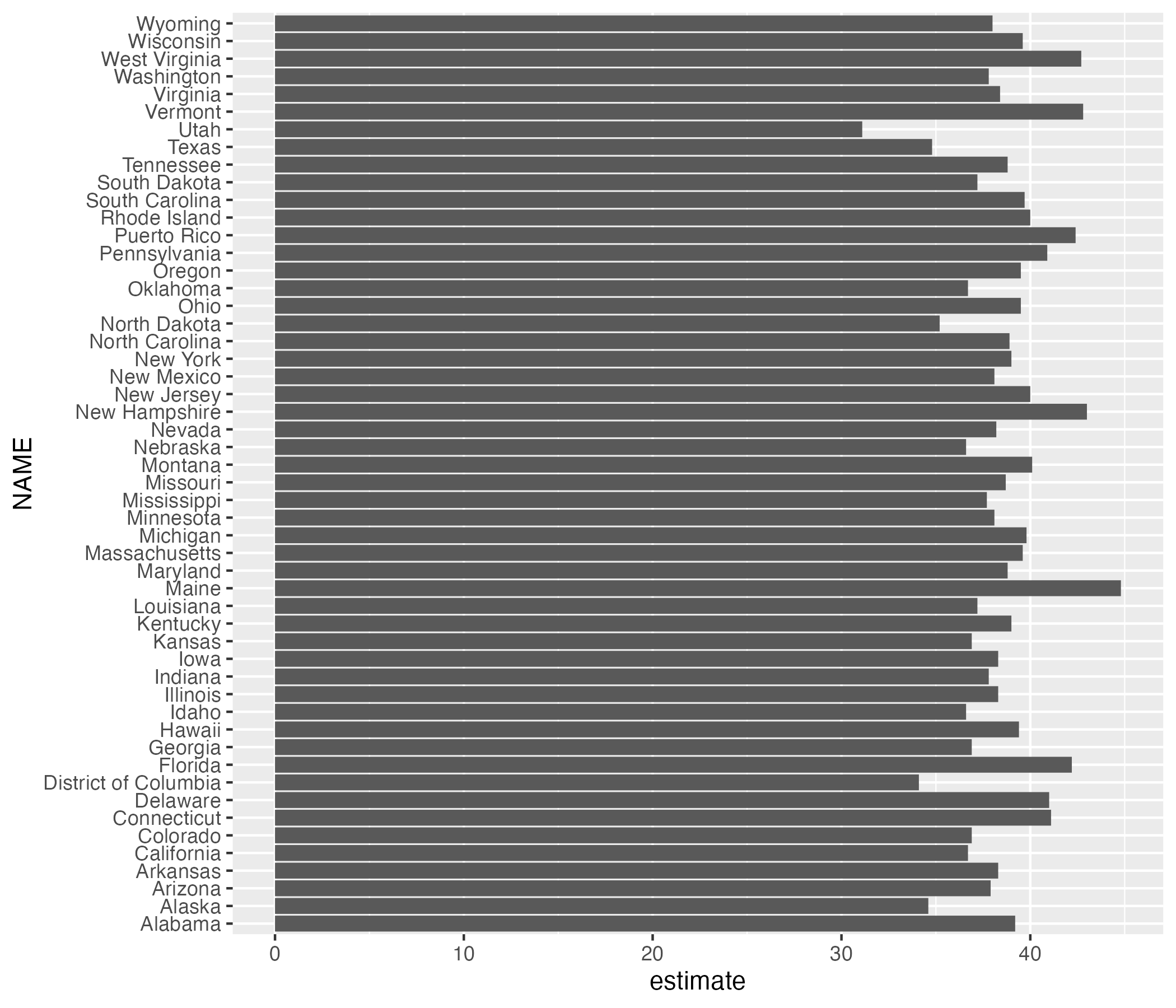
Figure 11.1: A bar chart showing the median age in each state

This chart is nothing special, but the fact that it takes just six lines of code to create most definitely is.

Using ACS Data to Make Maps

Kyle Walker’s original motivation to build tidycensus came from wanting to make it easy to access demographic data, just as he had done with geospatial data in the tigris package. He succeeded. And one additional benefit of Walker working on both packages is that there is a tight integration between them. Using the get_acs() function, you can set the geometry argument to TRUE and you will get both demographic and geospatial data (which, under the hood, actually comes from the tigris package).

get_acs(geography = "state",
        variables = "B01002_001",
        year = 2020,
        geometry = TRUE) 

If we take a look at the resulting data, we can see that it has the metadata and geometry column of simple features objects that we saw in Chapter 4.

#> Simple feature collection with 52 features and 5 fields
#> Geometry type: MULTIPOLYGON
#> Dimension:     XY
#> Bounding box:  xmin: -179.1489 ymin: 17.88328 xmax: 179.7785 ymax: 71.36516
#> Geodetic CRS:  NAD83
#> First 10 features:
#>    GEOID        NAME   variable estimate moe
#> 1     35  New Mexico B01002_001     38.1 0.1
#> 2     72 Puerto Rico B01002_001     42.4 0.2
#> 3     06  California B01002_001     36.7 0.1
#> 4     01     Alabama B01002_001     39.2 0.1
#> 5     13     Georgia B01002_001     36.9 0.1
#> 6     05    Arkansas B01002_001     38.3 0.2
#> 7     41      Oregon B01002_001     39.5 0.1
#> 8     28 Mississippi B01002_001     37.7 0.2
#> 9     08    Colorado B01002_001     36.9 0.1
#> 10    49        Utah B01002_001     31.1 0.1
#>                          geometry
#> 1  MULTIPOLYGON (((-109.0502 3...
#> 2  MULTIPOLYGON (((-65.23805 1...
#> 3  MULTIPOLYGON (((-118.6044 3...
#> 4  MULTIPOLYGON (((-88.05338 3...
#> 5  MULTIPOLYGON (((-81.27939 3...
#> 6  MULTIPOLYGON (((-94.61792 3...
#> 7  MULTIPOLYGON (((-123.6647 4...
#> 8  MULTIPOLYGON (((-88.50297 3...
#> 9  MULTIPOLYGON (((-109.0603 3...
#> 10 MULTIPOLYGON (((-114.053 37...

We can pipe this data into ggplot to make a map with the following code.

get_acs(geography = "state",
        variables = "B01002_001",
        year = 2020,
        geometry = TRUE) %>% 
  ggplot(aes(fill = estimate)) +
  geom_sf() +
  scale_fill_viridis_c()

The resulting map, seen in Figure 11.2 below, is less than ideal. The problem with it is that the Aleutian Islands in Alaska cross the 180-degree line of longitude, also known as the international date line. As a result, most of Alaska is on one side of the map while a small part is on the other side. What’s more, both Hawaii and Puerto Rico, both being decently far from the United States mainland and relatively small, are hard to see.

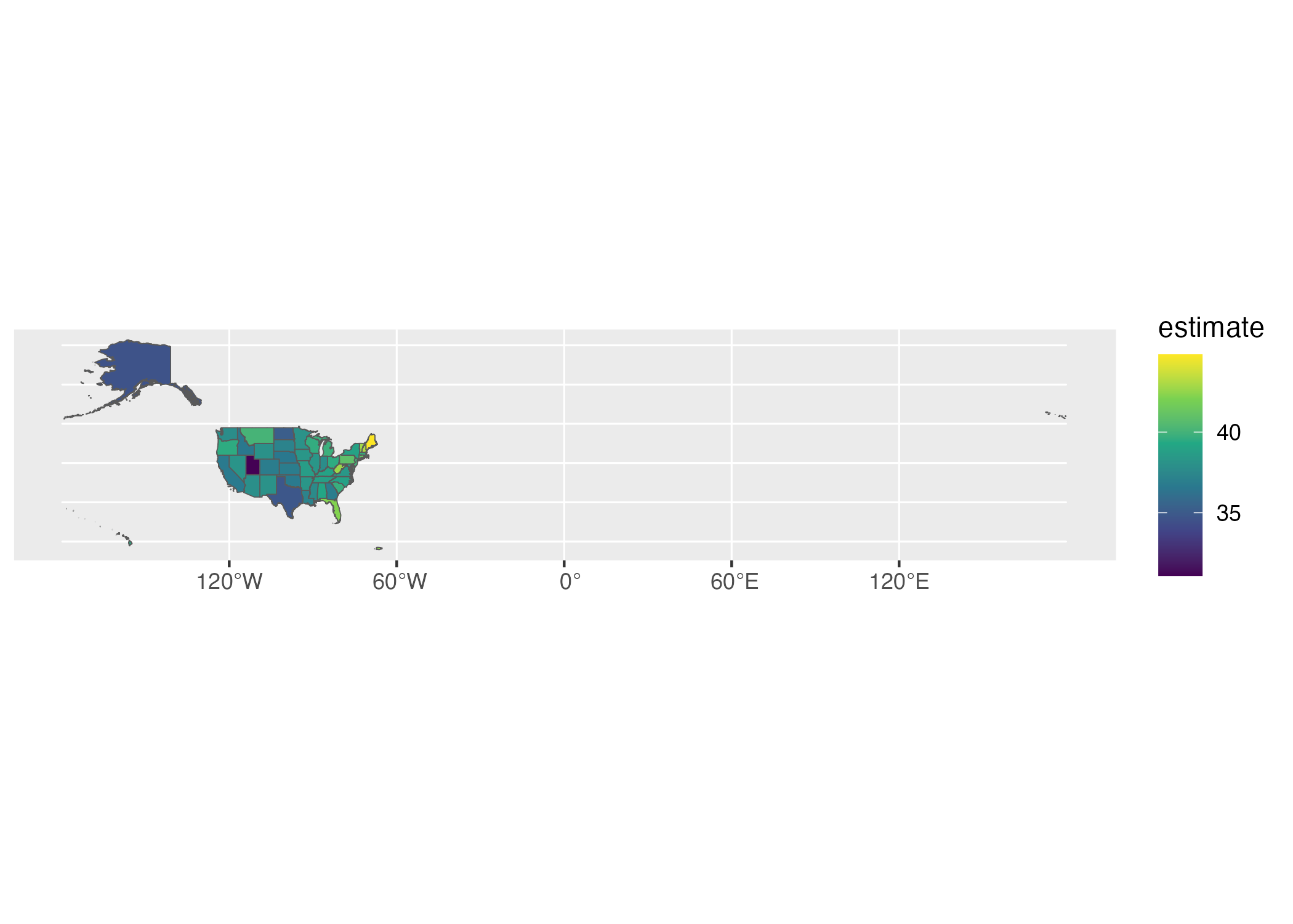
Figure 11.2: A hard-to-read map showing median age by state

Fortunately for us, Kyle Walker has a solution. If we load the tigris package, we can then use the shift_geometry() function to move Alaska, Hawaii, and Puerto Rico into places where they are more easily visible. We set the argument preserve_area to FALSE so that the giant state of Alaska is shrunk while Hawaii and Puerto Rico are made larger.

library(tigris)

get_acs(geography = "state",
        variables = "B01002_001",
        year = 2020,
        geometry = TRUE) %>% 
  shift_geometry(preserve_area = FALSE) %>% 
  ggplot(aes(fill = estimate)) +
  geom_sf() +
  scale_fill_viridis_c()

This lack of precision in the exact sizes of the states is more than made up for by having an easier to read map, which we can see in Figure 11.3.

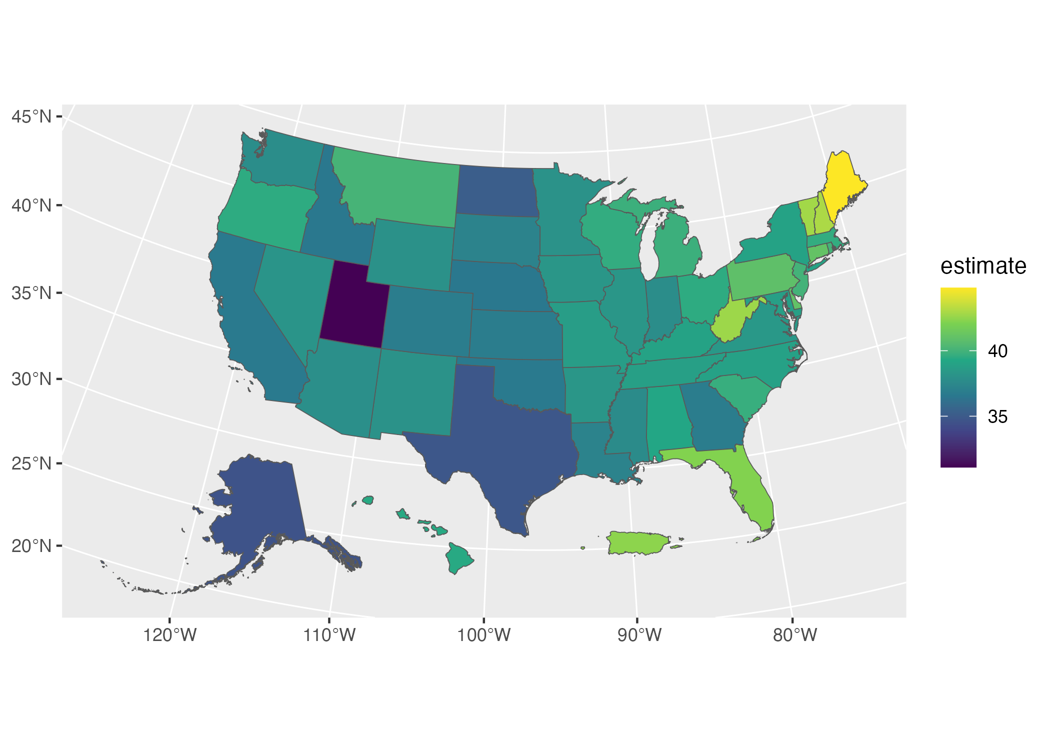
Figure 11.3: An easier-to-read map showing median age by state

We’ve made a map that shows median age by state. But there’s nothing to stop us from making the same map by county. Just change the geography argument to “county” and you’ll get a map for all 3,000 plus counties. Chapter 2 of Kyle Walker’s book Analyzing US Census Data: Methods, Maps, and Models in R discusses the various geographies available. There are also many more arguments in both the get_decennial() and get_acs() functions. We’ve only shown a few of the most common arguments. If you want to learn more, Walker’s book is a great resource.

In Conclusion: tidycensus Takes Care of the Tedious Parts of Working with Census Data

If you work with Census data, the tidycensus package is a huge timesaver. Rather than having to manually download data from the Census Bureau website, you can write R code that brings it in automatically, making it ready for analysis and reporting.

If you’re looking for Census data from other countries, Chapter 12 of Walker’s Analyzing US Census Data book gives examples of packages that can help. There are R packages to bring Census data from Canada, Kenya, Mexico, Brazil, and other countries.

What all of these packages (and the googlesheets4 package discussed in Chapter 10) have in common is that they use application programming interfaces (APIs) to access data directly from its source. These packages are often referred to as “wrapper packages” because they wrap R code around the code needed to access data through APIs. You don’t have to figure out how to access data through APIs yourself; you can just write some simple R code and the wrapper packages convert your code into the complex code needed to bring in the data.

In talking with Kyle Walker, he nicely summarized the benefit of tidycensus, saying it does “all of the tedious aspects of getting census data so that you can focus on the fun aspects.” He continued: “making maps is fun, analyzing data and finding out insights about your community is fun and interesting. But setting up a connector to an API or figuring out how to align columns [is] more tedious.”

This is the benefit of working with an open source tool like R. Because R is extensible, others can create packages to do things that would take you extraordinary amounts of time to do on your own. You don’t need to figure on your own out how to access the Census Bureau API by yourself. You can simply take advantage of the hours of work done by Kyle Walker and get all of the benefits of the tidycensus package.