10 Reproducible Reporting with Quarto
Quarto, the next-generation version of R Markdown, offers a few advantages over R Markdown. First, the syntax it uses across output types is more consistent. As you’ve seen in this book, R Markdown documents might use a variety of conventions; for example, the distill package has layout options that don’t work in xaringan, and xaringan uses three dashes to indicate new slides, while three dashes in other output formats would create a horizontal line.
Quarto also supports more languages than does R Markdown, as well as multiple code editors. While R Markdown is designed to work in the RStudio IDE, Quarto works in RStudio as well as code editors such as VS Code and JupyterLab, making it easy to use with multiple languages.
This chapter focuses on the benefits of using Quarto as an R user. It explains how to set up Quarto, then covers some of the most important differences between Quarto and R Markdown. Lastly, you’ll learn how to make the parameterized reports, presentations, and websites covered in previous chapters using Quarto.
Creating a Quarto Document
Versions of RStudio starting with 2022.07.1 come with Quarto installed. To check your RStudio version, click RStudio in the top menu bar, then click About RStudio. If you have an older version of RStudio, update it now by reinstalling it, as outlined in Chapter 1. Quarto should then be installed for you.
Once you’ve installed Quarto, create a document by clicking File > New File > Quarto Document. You should see a menu, shown in Figure 10.1, that looks like the one used to create an R Markdown document.
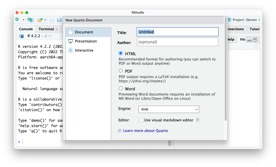
Figure 10.1: The RStudio menu for creating a new Quarto document
Give your document a title and choose an output format. The Engine option allows you to select a different way to render documents. By default, it uses Knitr, the same rendering tool used by R Markdown. The Use visual markdown editor option provides an interface that looks more like Microsoft Word, but it can be finicky, so we won’t cover it here.
The resulting Quarto document should contain default content, as do R Markdown documents:
---
title: "My Report"
format: html
---

## Quarto

Quarto enables you to weave together content and executable code into a finished document. To learn more about Quarto see <https://quarto.org>.

## Running Code

When you click the **Render** button a document will be generated that includes both content and the output of embedded code. You can embed code like this:

```{r}
1 + 1
```

You can add options to executable code like this

```{r}
#| echo: false
2 * 2
```

The `echo: false` option disables the printing of code (only output is displayed).
Although R Markdown and Quarto have many things in common, they also have differences. Let’s explore them.
Comparing R Markdown and Quarto
Quarto and R Markdown documents have the same basic structure: YAML metadata, followed by a combination of Markdown text and code chunks. Despite the similarities between the formats, there are some variations in their syntax.
The format and execute YAML Fields
Quarto uses slightly different options in its YAML. It replaces the output field with the format field and uses the value html instead of html_document:
---
title: "My Report"
output: html_document
---
Other Quarto formats also use slightly different names than their R Markdown counterparts: docx instead of word_document and pdf instead of pdf_document, for example.
A second difference between R Markdown and Quarto is that Quarto doesn’t use a setup code chunk to set default options about things like whether to show code, charts, and other elements in the rendered versions of the document. In Quarto, these options are set in the execute field of the YAML. For example, the following would hide code, as well as all warnings and messages, from the rendered document:
---
title: "My Report"
format: html
execute:
  echo: false
  warning: false
  message: false
---
Quarto also allows you to write true and false in lower case.
Individual Code Chunk Options
In R Markdown, we override options at the individual code chunk level by adding the new option within the curly brackets that start a code chunk. For example, the following would show both the code 2 * 2 as well as its output:
Quarto instead uses the following syntax to set individual code chunk-level options:
You can see that the option is set within the code chunk itself. The characters #| (known as the hash pipe) at the start of a line indicate that we are setting options.
Dashes in Option Names
Another difference you’re likely to see if you switch from R Markdown to Quarto is that option names consisting of two words are separated by a dash rather than a period. R Markdown, for example, uses the code chunk option fig.height to determine the height of plots. In contrast, Quarto uses fig-height, as follows:
```{r}
#| fig-height: 10

library(palmerpenguins)
library(tidyverse)

ggplot(
  penguins,
  aes(
    x = bill_length_mm,
    y = bill_depth_mm
  )
) +
  geom_point()
```
Helpfully for those of us coming from R Markdown, fig.height and similar options with periods in them will continue to work if you forget to make the switch. A list of all code chunk options can be found on the Quarto website at https://quarto.org/docs/reference/cells/cells-knitr.html.
The Render Button
You can follow the same process to render your Quarto document as in R Markdown, but in Quarto the button is called Render rather than Knit. Figure 10.2 shows the Render button.
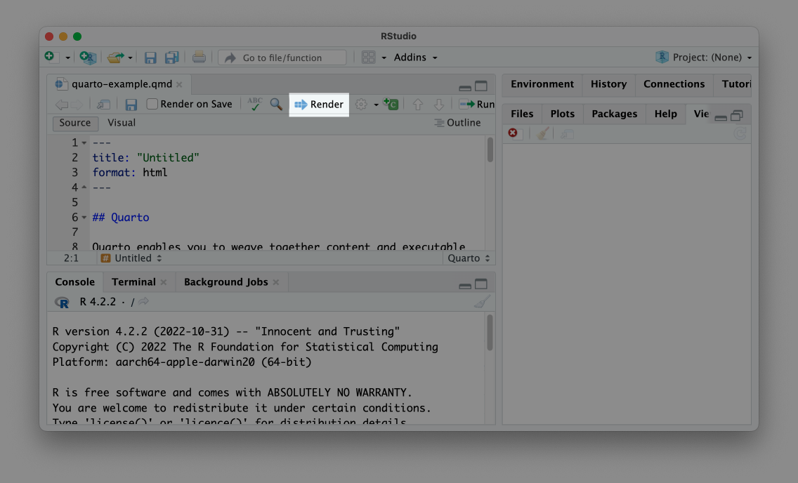
Figure 10.2: The Render button
Clicking the Render button will turn the Quarto document into an HTML file, Word document, or any other output format you select, just as we did when working with R Markdown.
Parameterized Reporting
Now that you’ve learned how Quarto works, let’s make a few different documents with it, starting with a parameterized report. The process of making parameterized reports with Quarto is nearly identical to doing so with R Markdown. In fact, you can take the R Markdown document used to make the Urban Institute COVID Report in Chapter 7 and adapt it for Quarto by copying the .Rmd file and changing its extension to .qmd, then making a few changes:
---
title: "Urban Institute COVID Report"
format: html
params:
  state: "Alabama"
execute:
  echo: false
  warning: false
  message: false
---

```{r}
library(tidyverse)
library(urbnthemes)
library(here)
library(scales)
```

# `r params$state`

```{r}
cases <- tibble(state.name) %>%
  rbind(state.name = "District of Columbia") %>%
  left_join(
    read_csv("https://data.rwithoutstatistics.com/united_states_covid19_cases_deaths_and_testing_by_state.csv", skip = 2),
    by = c("state.name" = "State/Territory")
  ) %>%
  select(
    total_cases = `Total Cases`,
    state.name,
    cases_per_100000 = `Case Rate per 100000`
  ) %>%
  mutate(cases_per_100000 = parse_number(cases_per_100000)) %>%
  mutate(case_rank = rank(-cases_per_100000, ties.method = "min"))
```

```{r}
state_text <- if_else(params$state == "District of Columbia", str_glue("the District of Columbia"), str_glue("state of {params$state}"))

state_cases_per_100000 <- cases %>%
  filter(state.name == params$state) %>%
  pull(cases_per_100000) %>%
  comma()

state_cases_rank <- cases %>%
  filter(state.name == params$state) %>%
  pull(case_rank)
```

In `r state_text`, there were `r state_cases_per_100000` cases per 100,000 people in the last seven days. This puts `r params$state` at number `r state_cases_rank` of 50 states and the District of Columbia.

```{r}
#| fig-height: 8

set_urbn_defaults(style = "print")

cases %>%
  mutate(highlight_state = if_else(state.name == params$state, "Y", "N")) %>%
  mutate(state.name = fct_reorder(state.name, cases_per_100000)) %>%
  ggplot(aes(
    x = cases_per_100000,
    y = state.name,
    fill = highlight_state
  )) +
  geom_col() +
  scale_x_continuous(labels = comma_format()) +
  theme(legend.position = "none") +
  labs(
    y = NULL,
    x = "Cases per 100,000"
  )
```
In this code, we’ve switched output: html_document to format: html in the YAML, We’ve also removed the setup code chunk and put the options that were there in the YAML. Lastly, we’ve switched the fig.height option in the last code chunk to fig-height and used the hash pipe to label it as an option.
Next, to create one report for each state, we must tweak the render.R script file we used to make parameterized reports in Chapter 7:
# Load packages
library(tidyverse)
library(quarto)

# Create a vector of all states and the District of Columbia
state <- tibble(state.name) %>%
  rbind("District of Columbia") %>%
  pull(state.name)

# Create a tibble with information on the:
# input R Markdown document
# output HTML file
# parameters needed to knit the document
reports <- tibble(
  input = "urban-covid-budget-report.qmd",
  output_file = str_glue("{state}.html"),
  execute_params = map(state, ~list(state = .))
)

# Generate all of our reports
reports %>%
  pwalk(quarto_render)
This updated render.R file loads the quarto package instead of the rmarkdown package and changes the input file to urban-covid-budget-report.qmd. In the reports tibble, we use execute_params instead of params because this is the argument that the quarto_render() function expects. To render the reports, we use the quarto_render() function instead of the render() function from the markdown package. As in Chapter 7, running this code should produce one report for each state.
Making Presentations
Quarto can produce presentations like those you made in Chapter 8 with the xaringan package. To make a presentation with Quarto, click File > New File > Quarto Presentation. Choose Reveal JS to make your slides and leave the Engine and Editor options untouched, as shown in Figure 10.3.
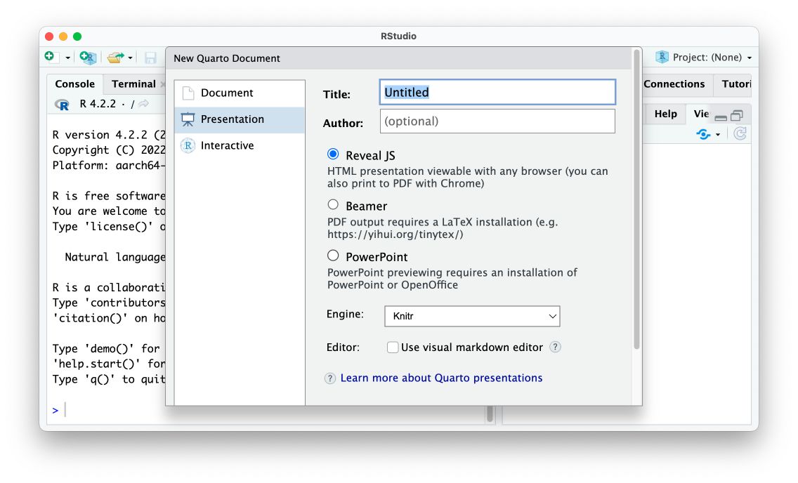
Figure 10.3: The RStudio menu to make a new Quarto presentation
The slides we’ll make use the reveal.js JavaScript library under the hood, a technique similar to making slides with xaringan. The following code updates the presentation made in Chapter 8 so it works with Quarto:
---
title: "Penguins Report"
author: "David Keyes"
format: revealjs
execute:
  echo: false
  warning: false
  message: false
---

# Introduction

```{r}
library(tidyverse)
```

```{r}
penguins <- read_csv("https://raw.githubusercontent.com/rfortherestofus/r-without-statistics/main/data/penguins-2008.csv")
```

We are writing a report about the **Palmer Penguins**. These penguins are *really* amazing. There are three species:

- Adelie
- Gentoo
- Chinstrap

## Bill Length

We can make a histogram to see the distribution of bill lengths.

```{r}
penguins %>%
  ggplot(aes(x = bill_length_mm)) +
  geom_histogram() +
  theme_minimal()
```

```{r}
average_bill_length <- penguins %>%
  summarize(avg_bill_length = mean(
    bill_length_mm,
    na.rm = TRUE
  )) %>%
  pull(avg_bill_length)
```

The chart shows the distribution of bill lengths. The average bill length is `r average_bill_length` millimeters.
In the YAML, we set format: revealjs to make a presentation and add several global code chunk options in the execute section. We remove the three dashes used to make slide breaks, because in Quarto, first- or second-level headings make new slides (though you can use three dashes to manually add slide breaks). When you render this code, you should get an HTML file with your slides. The output should look similar to the default xaringan slides we made.
Incrementally Revealing Content
Quarto slides can incrementally reveal content. To reveal bulleted and numbered lists one item at a time by default, add incremental: true to the document’s YAML:
---
title: "Penguins Report"
author: "David Keyes"
format:
  revealjs:
      incremental: true
execute:
  echo: false
  warning: false
  message: false
---
As a result, the content in all lists in the presentation should appear on the slide one item at a time. You can also set just some lists to incrementally reveal using this format:
Using ::: to start and end a segment of the document creates a section in the resulting HTML file known as a <div>. The HTML <div> tag allows you to define properties within that section. In this code, adding {.incremental} sets a custom CSS class that makes the list reveal incrementally.
Aligning Content and Adding Background Images
We can use ato create columns in Quarto slides, too. Let’s say we want to create a slide with content in two columns, as in Figure 10.4.
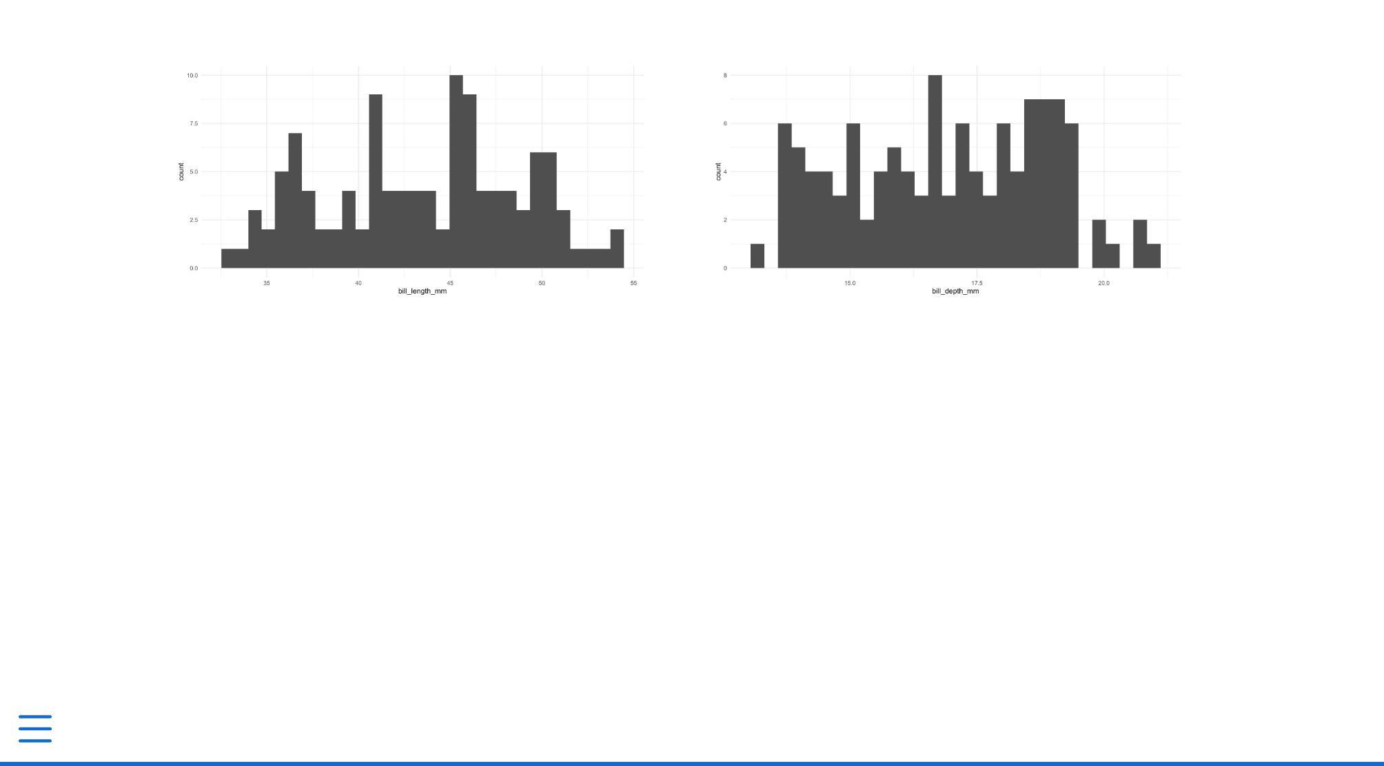
Figure 10.4: A slide with two columns
The following code created this two-column slide:
:::: {.columns}

::: {.column width="50%"}
```{r}
penguins %>%
  ggplot(aes(x = bill_length_mm)) +
  geom_histogram() +
  theme_minimal()
```

:::

::: {.column width="50%"}
```{r}
penguins %>%
  ggplot(aes(x = bill_depth_mm)) +
  geom_histogram() +
  theme_minimal()
```

:::

::::
Notice the :::, as well as ::::, which creates nested <div> sections. We first use a columns class, which tells the HTML that all content within the :::: should be laid out as columns. Then, we use ::: {.column width="50%"} to start a <div> that takes up half the width of the slide. With use closing :::: and ::: to indicate the end of the section.
When using xaringan, we easily centered content on a slide by surrounding it with .center[]. Doing the same thing in Quarto is slightly more complicated. Quarto has no built-in CSS class to center content, so we need to create one ourselves. Begin a CSS code chunk and a custom class called center-slide:
Using CSS, we center-align all content. (The text-align property aligns images, too, not just text.) We then apply the new center-slide class by putting it next to the title of the slide, as follows:
With the custom CSS applied, the slide should now center all content.
Lastly, when working in xaringan, we added a background image to a slide. We can do the same thing in Quarto by applying the background-image attribute to a slide, as follows:
This should add a slide with the text Penguins in front of the selected image.
Customizing Your Slides with Themes and CSS
We’ve started making some changes to the look-and-feel of the Quarto slides. As with xaringan, there are two main ways to further customize your slides: using existing themes and changing the CSS.
Themes are the easiest way to change what your slides look like. Quarto has many themes you can apply by adding their name to your YAML, as follows:
Using this option should change the theme from the default of light to a dark theme. You can see the title slide with the dark theme applied in Figure 10.5. To see the full list of available themes, go to https://quarto.org/docs/presentations/revealjs/themes.html.

Figure 10.5: A slide with the dark theme applied
You can also write custom CSS to change your slides further. Quarto uses a type of CSS called Sass that lets us include variables in the CSS. These variables resemble those from the xaringanthemer package, which allowed us to set values for header formatting using header_h2_font_size and header_color.
Go to File > New File > New Text File, create a Sass file called theme.scss, and add the following two mandatory sections to it as follows:
In the scss:defaults section, we can use the Quarto Sass variables. For example, to change the color and size of first-level headers, add this code:
/*-- scss:defaults --*/
$presentation-heading-color: red;
$presentation-h1-font-size: 150px;

/*-- scss:rules --*/
All Quarto Sass variables start with a dollar sign, followed by a name. To apply these tweaks to your slides, adjust your YAML to tell Quarto use the custom theme.scss file:
Figure 10.6 shows the changes applied to the rendered slides.
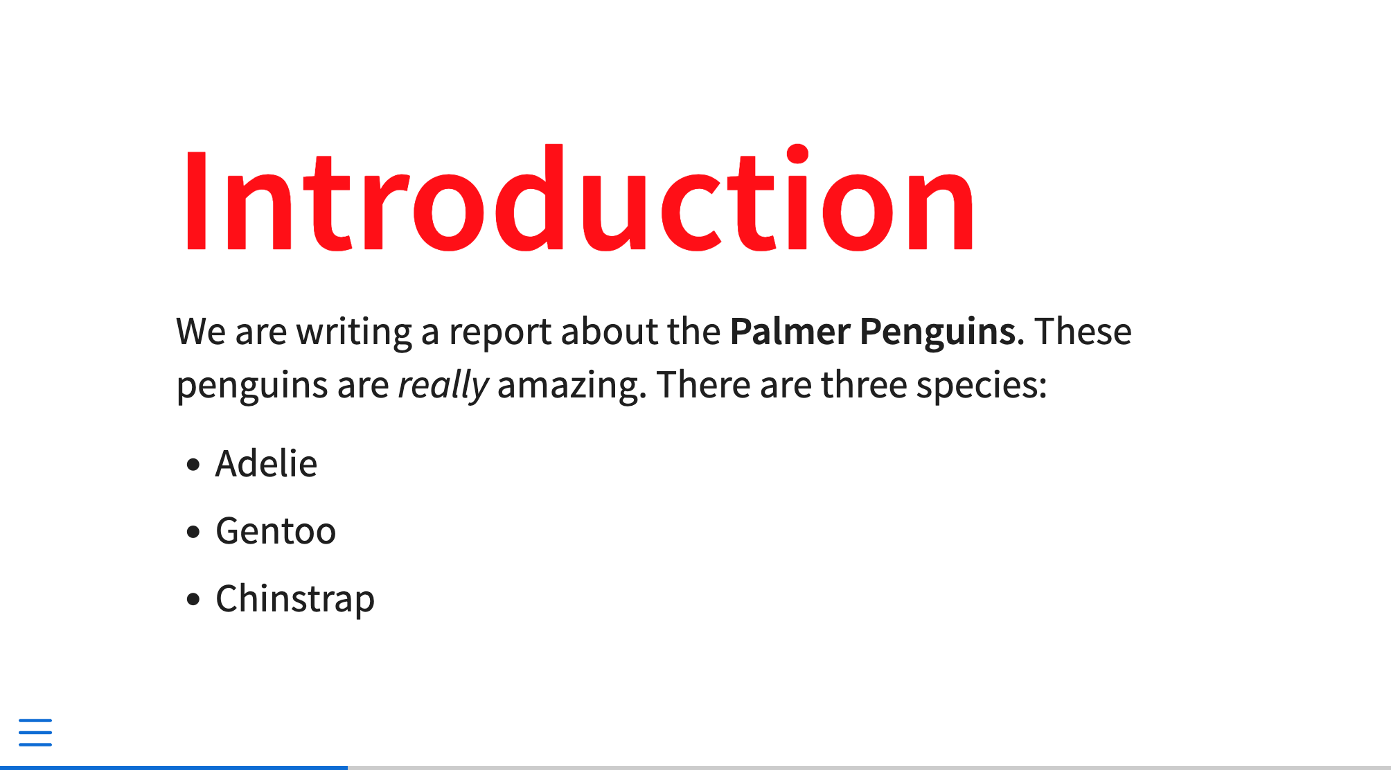
Figure 10.6: A slide with custom CSS applied to it
All pre-defined variables should go in the scss:defaults section, and you can find the full list of variables at https://quarto.org/docs/presentations/revealjs/themes.html#sass-variables. In the sass:rules section, you can add additional CSS tweaks for which there are no existing variables. For example, you could place the code you wrote to center the slide’s content in this section:
/*-- scss:defaults --*/
$presentation-heading-color: red;
$presentation-h1-font-size: 150px;

/*-- scss:rules --*/
.center-slide {
  text-align: center;
}
Because rendered Quarto slides are HTML documents, you can tweak them however you would like with custom CSS. What’s more, because the slides use reveal.js under the hood, any features built into that JavaScript library work in Quarto. This library includes easy ways to add transitions, animations, interactive content, and much more. The demo Quarto presentation available at https://quarto.org/docs/presentations/revealjs/demo/ shows many of these features in action.
Making Websites
Quarto can make websites without requiring the use of an external package like distill. To create a Quarto website, go to File > New Project. Select New Directory, then Quarto website. You’ll be prompted to choose a directory in which to place your project. Keep the default engine (Knitr), check Create a git repository (which should show up only if you’ve already installed git). and leave everything else unchecked. Your screen should look like Figure 10.7.
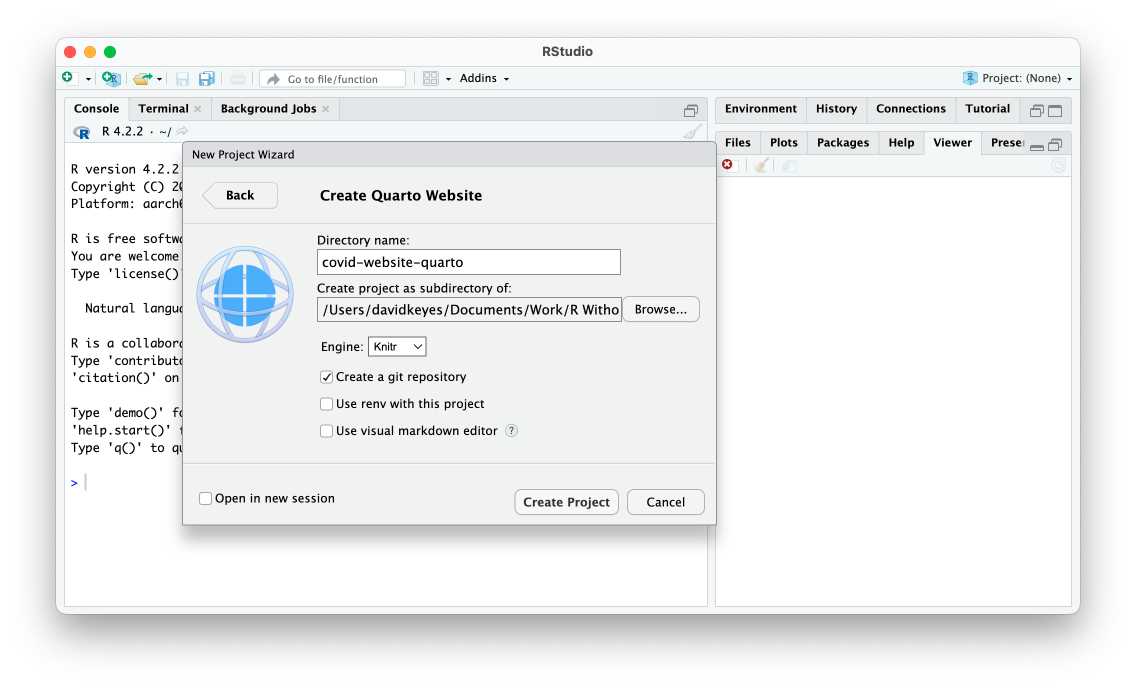
Figure 10.7: The RStudio menu to create a Quarto website
Click Create Project, which should create a series of files: index.qmd, about.qmd, *_quarto.yml, and styles.css. These files resemble those created by the distill package. The .qmd files are where we’ll add content, the _quarto.yml* file is where we’ll set options for the entire website, and the styles.css file is where we’ll add CSS to customize the website’s appearance.
Building the Website
Let’s start by modifying the .qmd files. Open the home page file, index.qmd, delete the default content below the YAML and replace it with the content from website you made in Chapter 9. Remove the layout = "l-page" element, which we used to widen the layout. We’ll discuss how to change the page’s layout in Quarto later in this section:
```{r}
# Load packages

library(tidyverse)
library(janitor)
library(tigris)
library(gt)
library(lubridate)
library(reactable)
```

```{r}
# Import data

us_states <- states(
  cb = TRUE,
  resolution = "20m",
  progress_bar = FALSE
) %>%
  shift_geometry() %>%
  clean_names() %>%
  select(geoid, name) %>%
  rename(state = name) %>%
  filter(state %in% state.name)

covid_data <- read_csv("https://raw.githubusercontent.com/nytimes/covid-19-data/master/rolling-averages/us-states.csv") %>%
  filter(state %in% state.name) %>%
  mutate(geoid = str_remove(geoid, "USA-"))

most_recent_day <- covid_data %>%
  slice_max(
    order_by = date,
    n = 1
  ) %>%
  distinct(date) %>%
  mutate(date_nice_format = str_glue("{month(date, label = TRUE, abbr = FALSE)} {day(date)}, {year(date)}")) %>%
  pull(date_nice_format)
```

# COVID Death Rates as of `r most_recent_day`

This table shows COVID death rates per 100,000 people in four states states.

```{r}
# Make table

covid_data %>%
  slice_max(
    order_by = date,
    n = 1
  ) %>%
  select(state, deaths_avg_per_100k) %>%
  arrange(state) %>%
  set_names("State", "Death rate") %>%
  reactable()
```

We can see this same death rate data for all states on a map.

```{r}
# Make map

most_recent <- us_states %>%
  left_join(covid_data, by = "state") %>%
  slice_max(
    order_by = date,
    n = 1
  )

most_recent %>%
  ggplot(aes(fill = deaths_avg_per_100k)) +
  geom_sf() +
  scale_fill_viridis_c(option = "rocket") +
  labs(fill = "Deaths per\n100,000 people") +
  theme_void()
```

# COVID Death Rates Over Time

The following chart shows COVID death rates from the start of COVID in early 2020 until `r most_recent_day`.

```{r}
# Make chart

library(plotly)

covid_chart <- covid_data %>%
  filter(state %in% c(
    "Alabama",
    "Alaska",
    "Arizona",
    "Arkansas"
  )) %>%
  ggplot(aes(
    x = date,
    y = deaths_avg_per_100k,
    group = state,
    fill = deaths_avg_per_100k
  )) +
  geom_col() +
  scale_fill_viridis_c(option = "rocket") +
  theme_minimal() +
  labs(title = "Deaths per 100,000 people over time") +
  theme(
    legend.position = "none",
    plot.title.position = "plot",
    plot.title = element_text(face = "bold"),
    panel.grid.minor = element_blank(),
    axis.title = element_blank()
  ) +
  facet_wrap(
    ~state,
    nrow = 2
  )


ggplotly(covid_chart)
```
To render a Quarto website, look for the Build tab in the top right of RStudio and click Render Website. The rendered website should now appear in the Viewer pane on the bottom-right panel of RStudio. If you navigate to the Files pane on the same panel, you should also see that a _site folder has been created to hold the content of the rendered site. Try opening the index.html file in your web browser. You should see the website in Figure 10.8.
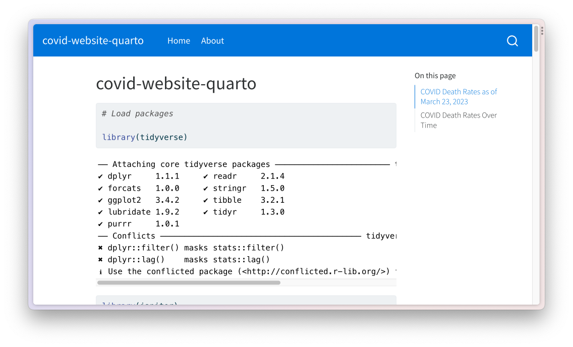
Figure 10.8: The Quarto website with warnings and messages
As you can see, the web page includes many warnings and messages that we don’t want to show. In R Markdown, we removed these in our setup code chunk; in Quarto, we can do this in the YAML. Add the following code to the index.qmd YAML to remove all code, warnings, and messages from the output:
Note, however, that these options will make changes to only one file. Next, we discuss how to set these options for the entire website.
Setting Options for the Website
When using distill, we modified the *_site.yml* file to make changes to all files in the website. In Quarto, we use the *_quarto.yml* file for the same purpose. If you open it, you should see three sections:
project:
type: website
website:
title: "covid-website-quarto"
navbar:
left:
- href: index.qmd
text: Home
- about.qmd
format:
html:
theme: cosmo
css: styles.css
toc: trueThe top section sets the project type (in this case, a website). The middle section defines the website’s title and determines the options for its navigation bar. The bottom section modifies the site’s appearance.
Let’s start from the bottom. To remove code, warnings, and messages for all pages in our website, add the portion of the YAML we created above to the _quarto.yml file. The bottom section should now look like this:
format:
html:
theme: cosmo
css: styles.css
toc: true
execute:
  echo: false
  warning: false
message: falseIf you build the website again, you should now see just the content, as in Figure 10.9.
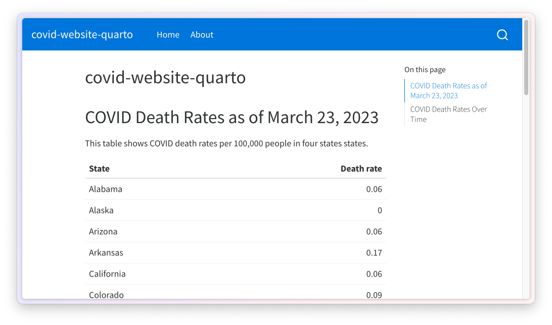
Figure 10.9: The website with warnings and messages removed
In this section of the *_quarto.yml* file, you can add any options you would otherwise place in a single .qmd file to apply them across all pages of your website.
Changing the Appearance of the Website with Themes and CSS
The format section of the *_quarto.yml* file determines the appearance of rendered files. By default, Quarto applies a theme called cosmo, but there are many themes available. (You can see the full list at https://quarto.org/docs/output-formats/html-themes.html.) Let’s apply a different theme to see how it affects the output:
Using the minty theme changes the colors and fonts on the website, as shown in Figure 10.10.
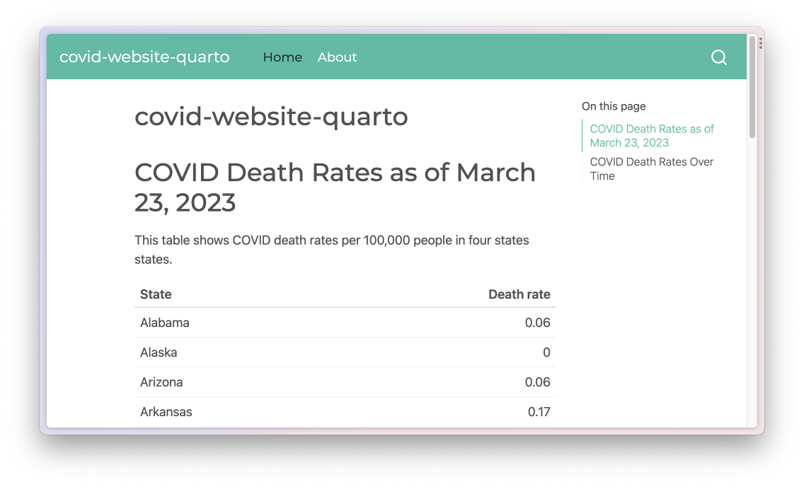
Figure 10.10: The website with the minty theme
In addition to using pre-built themes, you can customize your website with CSS. The css: styles.css section in the *_quarto.yml* file indicates that Quarto will use any CSS in the styles.css file when rendering. Try adding the following CSS to styles.css to make first-level headers red and 50 pixels large:
The re-rendered index.html, shown in Figure 10.11, now has large red headings.
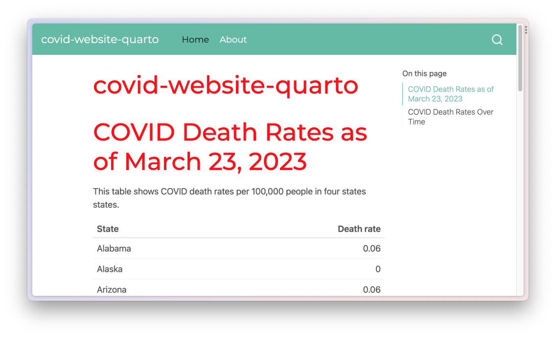
Figure 10.11: The website with custom CSS applied
An alternative approach to customizing your website is to use Sass variables in a .scss file, as you did in your presentation. For example, create a file called styles.scss and add a line like this one to make the body background bright yellow:
To get Quarto to use the styles.scss file, adjust the theme line as follows:
This syntax tells Quarto to use the minty theme, then make additional tweaks based on the styles.scss file. If you render the website again, you should see the bright yellow background throughout (Figure 10.12).
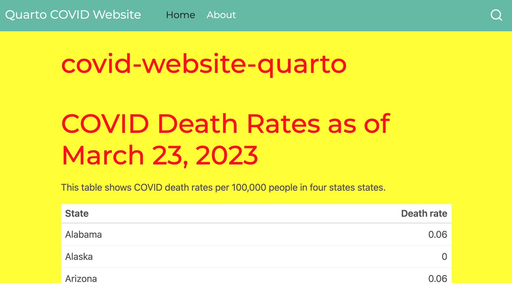
Figure 10.12: The website with custom CSS applied through styles.scss
Note that when you add a .scss file, the tweaks made in styles.css no longer apply. If you wanted to use those, you’d need to add them to the styles.scss file.
The line toc: true creates a table of contents on the right side of the web pages that you can see in the previous screenshots. You can remove it by changing true to false. Add any additional options, such as figure height, to the bottom section of the *_quarto.yml* file.
Adjusting the Website Title and Navigation Bar
The middle section of the *_quarto.yml* file sets the website’s title and navigation. Here, we change the title and the text for the About page link:
website:
  title: "Quarto COVID Website"
  navbar:
    left:
      - href: index.qmd
        text: Home
      - href: about.qmd
        text: About this Website
Changing the title requires adjusting the title line. The navbar section functions nearly identically to how it does when working with distill. The href line lists the files the navigation bar should link to. The optional text line specifies the text that should show up for that link. Figure 10.13 shows these changes applied to the website.

Figure 10.13: The website with changes to the navigation bar
The title on the home page is still covid-website-quarto, but you could change this in the index.qmd file.
Creating Wider Layouts
When we made a website with distill, we used the line layout = "l-page" to widen the map on the web page. We can accomplish the same thing with Quarto by using the::: syntax to add HTML <div> tags:
:::{.column-screen-inset}
```{r}
#| out-width: 100%
# Make map

most_recent <- us_states %>%
  left_join(covid_data, by = "state") %>%
  slice_max(
    order_by = date,
    n = 1
  )

most_recent %>%
  ggplot(aes(fill = deaths_avg_per_100k)) +
  geom_sf() +
  scale_fill_viridis_c(option = "rocket") +
  labs(fill = "Deaths per\n100,000 people") +
  theme_void()
```
:::
We add :::{.column-screen-inset} to the beginning of the code chunk that makes the map and ::: to the end of the code chunk. We also add the line #| out-width: 100% in the code chunk. This is because we need to specify that the map should take up all of the available width. Without this line, the map would take up only a portion of the window. There are a number of different output widths you can use. The full list is available at https://quarto.org/docs/authoring/article-layout.html.
Hosting Your Website on GitHub Pages and Quarto Pub
You can host your Quarto website using GitHub Pages, just as you did with your distill website. Recall that GitHub Pages requires you to save the website’s files in the docs folder. Change the *_quarto.yml* file so that the site outputs to this folder:
Now, when you render the site, the HTML and other files should show up in the docs directory. At this point, you can push your repository to GitHub, adjust the GitHub Pages settings as you did in Chapter 9, and receive a URL at which your Quarto website will live.
In addition to using GitHub Pages, Quarto has a free service called Quarto Pub that makes it easy to get your materials online. If you’re not a GitHub user, this is a great way to publish your work. To see how it works, let’s publish the website we just made to it. Click the Terminal tab on the bottom-left panel of RStudio. At the prompt, enter the text quarto publish and hit Enter. Doing so should bring up a list of ways you can publish your website, as in Figure 10.14.
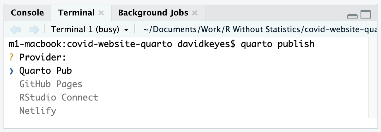
Figure 10.14: The list of providers to publish your Quarto website
Press Enter to select Quarto Pub. You’ll then be asked to authorize RStudio to publish to Quarto Pub. Enter Y to do so, which should take you to https://quartopub.com/. Sign up for an account (or sign in if you already have one). You should see a screen indicating that you have successfully signed in and authorized RStudio to connect with Quarto Pub. From there, you can return to RStudio, which should prompt you to select a name for your website. The easiest thing is to use your project’s name. Once you enter the name, Quarto Pub should publish the site and take you to it, as shown in Figure 10.15.
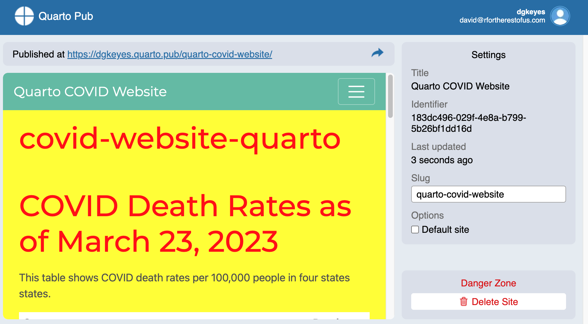
Figure 10.15: The website published on Quarto Pub
When you make updates to your site, you can republish it to Quarto Pub using the same steps. Quarto Pub is probably the easiest way to publish HTML files made with Quarto.
Conclusion
As you’ve seen in this chapter, you can do everything you did in R Markdown using Quarto without loading any external packages. In addition, Quarto’s different output formats use a more consistent syntax. For example, because you can make new slides in Quarto by adding first- or second-level headers, the Quarto documents you use to create reports should translate easily to presentations.
You’re probably wondering at this point whether you should use R Markdown or Quarto. It’s a big question, and one many in the R community are thinking about. The first thing to know is that R Markdown isn’t going away, so if you already use R Markdown, you don’t need to switch. If you’re new to R, however, you may be a good candidate for Quarto, as the R Markdown team has promised to continue its development, and its future features may not be backported to R Markdown.
Ultimately, the differences between R Markdown and Quarto are relatively small, and the impact of switching between tools should be minor. Both R Markdown and Quarto can help you become more efficient, avoid manual errors, and share results in a wide variety of formats.
Learn More
Consult the following resources to learn the fundamentals of Quarto:
Get Started with Quarto, workshop materials by Tom Mock (2022), https://jthomasmock.github.io/quarto-in-two-hours/
From R Markdown to Quarto, workshop materials by Andrew Bray, Rebecca Barter, Silvia Canelón, Christophe Dervieu, Devin Pastor, and Tatsu Shigeta (2022), https://rstudio-conf-2022.github.io/rmd-to-quarto/