12 Creating Functions and Packages
You are reading the free online version of this book. If you’d like to purchase a physical or electronic copy, you can buy it from No Starch Press, Powell’s, Barnes and Noble or Amazon.
In this chapter, you will learn how to define your own R functions, including the parameters they should accept. Then, you’ll create a package to distribute those functions, add your code and dependencies to it, write its documentation, and choose the license under which to release it.
Saving your code as custom functions and then distributing them in packages can have numerous benefits. First, packages make your code easier for others to use. For example, when researchers at the Moffitt Cancer Center needed to access code from a database, data scientists Travis Gerke and Garrick Aden-Buie used to write R code for each researcher, but they quickly realized they were reusing the same code over and over. Instead, they made a package with functions for accessing databases. Now researchers no longer had to ask for help; they could simply install the package Gerke and Aden-Buie had made and use its functions themselves.
What’s more, developing packages allows you to shape how others work. Say you make a ggplot theme that follows the principles of high-quality data visualization discussed in Chapter 3. If you put this theme in a package, you can give others an easy way to follow these design principles. In short, functions and packages help you work with others using shared code.
Creating Your Own Functions
Hadley Wickham, developer of the tidyverse set of packages, recommends creating a function once you’ve copied some code three times. Functions have three pieces: a name, a body, and arguments.
Writing a Simple Function
You’ll begin by writing an example of a relatively simple function. This function, called show_in_excel_penguins(), opens the penguin data from Chapter 7 in Microsoft Excel:
This code first loads the tidyverse and fs packages. You’ll use tidyverse to create a filename for the CSV file and save it, and fs to open the CSV file in Excel (or whichever program your computer uses to open CSV files by default).
Next, the read_csv() function imports the penguin data and names the data frame penguins. Then it creates the new show_in_excel_penguins function, using the assignment operator (<-) and function() to specify that show_in_excel_penguins isn’t a variable name but a function name. The open curly bracket ({) at the end of the line indicates the start of the function body, where the “meat” of the function can be found. In this case, the body does three things:
Creates a location for a CSV file to be saved using the
str_glue()function combined with thetempfile()function. This creates a file at a temporary location with the .csv extension and saves it ascsv_file.Writes penguins to the location set in
csv_file. Thexargument inwrite_csv()refers to the data frame to be saved. It also specifies that allNAvalues should show up as blanks. (By default, they would display the text NA.)Uses the
file_show()function from thefspackage to open the temporary CSV file in Excel.
To use the show_in_excel_penguins() function, highlight the lines that define the function and then press command-enter on macOS or ctrl-enter on Windows. You should now see the function in your global environment, as shown in Figure 12.1.
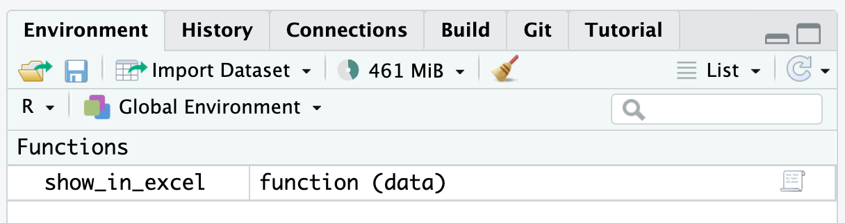
From now on, any time you run the code show_in_excel_penguins(), R will open the penguins data frame in Excel.
Adding Arguments
You’re probably thinking that this function doesn’t seem very useful. All it does is open the penguins data frame. Why would you want to keep doing that? A more practical function would let you open any data in Excel so you can use it in a variety of contexts.
The show_in_excel() function does just that: it takes any data frame from R, saves it as a CSV file, and opens the CSV file in Excel. Bruno Rodrigues, head of the Department of Statistics and Data Strategy at the Ministry of Higher Education and Research in Luxembourg, wrote show_in_excel() to easily share data with his non-R-user colleagues. Whenever he needed data in a CSV file, he could run this function.
Replace your show_in_excel_penguins() function definition with this slightly simplified version of the code that Rodrigues used:
This code looks the same as show_in_excel_penguins(), with two exceptions. Notice that the first line now says function(data). Items listed within the parentheses of the function definition are arguments. If you look farther down, you’ll see the second change. Within write_csv(), instead of x = penguins, it now says x = data. This allows you to use the function with any data, not just penguins.
To use this function, you simply tell show_in_excel() what data to use, and the function opens the data in Excel. For example, tell it to open the penguins data frame as follows:
show_in_excel(data = penguins)Having created the function with the data argument, now you can run it with any data you want to. This code, for example, imports the COVID case data from Chapter 4 and opens it in Excel:
covid_data <- read_csv("https://data.rfortherestofus.com/us-states-covid-rolling-average.csv")

show_in_excel(data = covid_data)
You can also use show_in_excel() at the end of a pipeline. This code filters the covid_data data frame to include only data from California before opening it in Excel:
Rodrigues could have copied the code within the show_in_excel() function and rerun it every time he wanted to view his data in Excel. But, by creating a function, he was able to write the code just once and then run it as many times as necessary.
Creating a Function to Automatically Format Race and Ethnicity Data
Hopefully now you better understand how functions work, so let’s walk through an example function you could use to simplify some of the activities from previous chapters.
In Chapter 11, when you used the tidycensus package to automatically import data from the US Census Bureau, you learned that the census data has many variables with nonintuitive names. Say you regularly want to access data about race and ethnicity from the American Community Survey, but you can never remember which variables enable you to do so. To make your task more efficient, you’ll create a get_acs_race_ethnicity() function step-by-step in this section, learning some important concepts about custom functions along the way.
A first version of the get_acs_race_ethnicity() function might look like this:
library(tidycensus)

get_acs_race_ethnicity <- function() {
  race_ethnicity_data <-
    get_acs(
      geography = "state",
      variables = c(
        "White" = "B03002_003",
        "Black/African American" = "B03002_004",
        "American Indian/Alaska Native" = "B03002_005",
        "Asian" = "B03002_006",
        "Native Hawaiian/Pacific Islander" = "B03002_007",
        "Other race" = "B03002_008",
        "Multi-Race" = "B03002_009",
        "Hispanic/Latino" = "B03002_012"
      )
    )

  race_ethnicity_data
}
Within the function body, this code calls the get_acs() function from tidycensus to retrieve population data at the state level. But instead of returning the function’s default output, it updates the hard-to-remember variable names to human-readable names, such as White and Black/African American, and saves them as an object called race_ethnicity_data. The code then uses the race_ethnicity_data object to return that data when the get_acs_race_ethnicity() function is run.
To run this function, enter the following:
get_acs_race_ethnicity()Doing so should return data with easy-to-read race and ethnicity group names:
# A tibble: 416 × 5
   GEOID NAME    variable                         estimate   moe
   <chr> <chr>   <chr>                               <dbl> <dbl>
 1 01    Alabama White                             3247262  2133
 2 01    Alabama Black/African American            1318388  3585
 3 01    Alabama American Indian/Alaska Native       14864   868
 4 01    Alabama Asian                               69099  1113
 5 01    Alabama Native Hawaiian/Pacific Islander     1557   303
 6 01    Alabama Other race                          14724  1851
 7 01    Alabama Multi-Race                         129791  3724
 8 01    Alabama Hispanic/Latino                    232407   199
 9 02    Alaska  White                              428802  1173
10 02    Alaska  Black/African American              22400   935
# ℹ 406 more rows
You could improve this function in a few ways. You might want the resulting variable names to follow a consistent syntax, for example, so you could use the clean_names() function from the janitor package to format them in snake case (in which all words are lowercase and separated by underscores). However, you might also want to have the option of keeping the original variable names. To accomplish this, add the clean_variable_names argument to the function definition as follows:
get_acs_race_ethnicity <- function(clean_variable_names = FALSE) {
  race_ethnicity_data <-
    get_acs(
      geography = "state",
      variables = c(
        "White" = "B03002_003",
        "Black/African American" = "B03002_004",
        "American Indian/Alaska Native" = "B03002_005",
        "Asian" = "B03002_006",
        "Native Hawaiian/Pacific Islander" = "B03002_007",
        "Other race" = "B03002_008",
        "Multi-Race" = "B03002_009",
        "Hispanic/Latino" = "B03002_012"
      )
    )

  if (clean_variable_names == TRUE) {
    race_ethnicity_data <- clean_names(race_ethnicity_data)
  }

  race_ethnicity_data
}
This code adds the clean_variable_names argument to get_acs_race _ethnicity() and specifies that its value should be FALSE by default. Then, in the function body, an if statement says that if the argument is TRUE, the variable names should be overwritten by versions formatted in snake case. If the argument is FALSE, the variable names remain unchanged.
If you run the function now, nothing should change, because the new argument is set to FALSE by default. Try setting clean_variable_names to TRUE as follows:
get_acs_race_ethnicity(clean_variable_names = TRUE)This function call should return data with consistent variable names:
# A tibble: 416 × 5
   geoid name    variable                         estimate   moe
   <chr> <chr>   <chr>                               <dbl> <dbl>
 1 01    Alabama White                             3247262  2133
 2 01    Alabama Black/African American            1318388  3585
 3 01    Alabama American Indian/Alaska Native       14864   868
 4 01    Alabama Asian                               69099  1113
 5 01    Alabama Native Hawaiian/Pacific Islander     1557   303
 6 01    Alabama Other race                          14724  1851
 7 01    Alabama Multi-Race                         129791  3724
 8 01    Alabama Hispanic/Latino                    232407   199
 9 02    Alaska  White                              428802  1173
10 02    Alaska  Black/African American              22400   935
# ℹ 406 more rows
Notice that GEOID and NAME now appear as geoid and name.
Now that you’ve seen how to add arguments to two separate functions, you’ll learn how to pass arguments from one function to another.
Using … to Pass Arguments to Another Function
The get_acs_race_ethnicity() function you’ve created retrieves population data at the state level by passing the geography = "state" argument to the get_acs() function. But what if you wanted to obtain county-level or census tract data? You could do so using get_acs(), but get_acs_race_ethnicity() isn’t currently written in a way that would allow this. How could you modify the function to make it more flexible?
Your first idea might be to add a new argument for the level of data to retrieve. You could edit the first two lines of the function as follows to add a my_geography argument and then use it in the get_acs() function like so:
get_acs_race_ethnicity <- function(
  clean_variable_names = FALSE,
  my_geography
) {
  race_ethnicity_data <-
    get_acs(
      geography = my_geography,
      variables = c(
        "White" = "B03002_003",
        "Black/African American" = "B03002_004",
        "American Indian/Alaska Native" = "B03002_005",
        "Asian" = "B03002_006",
        "Native Hawaiian/Pacific Islander" = "B03002_007",
        "Other race" = "B03002_008",
        "Multi-Race" = "B03002_009",
        "Hispanic/Latino" = "B03002_012"
      )
    )

  if (clean_variable_names == TRUE) {
    race_ethnicity_data <- clean_names(race_ethnicity_data)
  }

  race_ethnicity_data
}
But what if you also want to select the year for which to retrieve data? Well, you could add an argument for that as well. However, as you saw in Chapter 11, the get_acs() function has many arguments, and repeating them all in your code would quickly become cumbersome.
The ... syntax gives you a more efficient option. Placing ... in the get_acs_race_ethnicity() function allows you to automatically pass any of its arguments to get_acs() by including ... in that function as well:
get_acs_race_ethnicity <- function(
  clean_variable_names = FALSE,
  ...
) {
  race_ethnicity_data <-
    get_acs(
      ...,
      variables = c(
        "White" = "B03002_003",
        "Black/African American" = "B03002_004",
        "American Indian/Alaska Native" = "B03002_005",
        "Asian" = "B03002_006",
        "Native Hawaiian/Pacific Islander" = "B03002_007",
        "Other race" = "B03002_008",
        "Multi-Race" = "B03002_009",
        "Hispanic/Latino" = "B03002_012"
      )
    )

  if (clean_variable_names == TRUE) {
    race_ethnicity_data <- clean_names(race_ethnicity_data)
  }

  race_ethnicity_data
}
Try running your function by passing it the geography argument set to “state”:
get_acs_race_ethnicity(geography = "state")This should return the following:
# A tibble: 416 × 5
   GEOID NAME    variable                         estimate   moe
   <chr> <chr>   <chr>                               <dbl> <dbl>
 1 01    Alabama White                             3247262  2133
 2 01    Alabama Black/African American            1318388  3585
 3 01    Alabama American Indian/Alaska Native       14864   868
 4 01    Alabama Asian                               69099  1113
 5 01    Alabama Native Hawaiian/Pacific Islander     1557   303
 6 01    Alabama Other race                          14724  1851
 7 01    Alabama Multi-Race                         129791  3724
 8 01    Alabama Hispanic/Latino                    232407   199
 9 02    Alaska  White                              428802  1173
10 02    Alaska  Black/African American              22400   935
# ℹ 406 more rows
You’ll see that the GEOID and NAME variables are uppercase because the clean_variable_names argument is set to FALSE by default, and we didn’t change it when using the get_acs_race_ethnicity() function.
Alternatively, you could change the value of the argument to get data by county:
get_acs_race_ethnicity(geography = "county")You could also run the function with the geometry = TRUE argument to return geospatial data alongside demographic data:
get_acs_race_ethnicity(
  geography = "county",
  geometry = TRUE
)
The function should return data like the following:
Simple feature collection with 416 features and 5 fields
Geometry type: MULTIPOLYGON
Dimension:     XY
Bounding box:  xmin: -179.1467 ymin: 17.88328 xmax: 179.7785 ymax: 71.38782
Geodetic CRS:  NAD83
First 10 features:
   GEOID         NAME                         variable estimate  moe
1     35   New Mexico                            White   752424 1849
2     35   New Mexico           Black/African American    37996 1116
3     35   New Mexico    American Indian/Alaska Native   178608 1339
4     35   New Mexico                            Asian    32214  868
5     35   New Mexico Native Hawaiian/Pacific Islander     1117  190
6     35   New Mexico                       Other race     7680  967
7     35   New Mexico                       Multi-Race    50798 2565
8     35   New Mexico                  Hispanic/Latino  1051626   NA
9     46 South Dakota                            White   718056  978
10    46 South Dakota           Black/African American    19172  805
                         geometry
1  MULTIPOLYGON (((-109.0502 3...
2  MULTIPOLYGON (((-109.0502 3...
3  MULTIPOLYGON (((-109.0502 3...
4  MULTIPOLYGON (((-109.0502 3...
5  MULTIPOLYGON (((-109.0502 3...
6  MULTIPOLYGON (((-109.0502 3...
7  MULTIPOLYGON (((-109.0502 3...
8  MULTIPOLYGON (((-109.0502 3...
9  MULTIPOLYGON (((-104.0579 4...
10 MULTIPOLYGON (((-104.0579 4...
The ... syntax allows you to create your own function and pass arguments from it to another function without repeating all of that function’s arguments in your own code. This approach gives you flexibility while keeping your code concise.
Now let’s look at how to put your custom functions into a package.
Creating a Package
Packages bundle your functions so you can use them in multiple projects. If you find yourself copying functions from one project to another, or from a functions.R file into each new project, that’s a good indication that you should make a package.
While you can run the functions from a functions.R file in your own environment, this code might not work on someone else’s computer. Other users may not have the necessary packages installed, or they may be confused about how your functions’ arguments work and not know where to go for help. Putting your functions in a package makes them more likely to work for everyone, as they include the necessary dependencies as well as built-in documentation to help others use the functions on their own.
Starting the Package
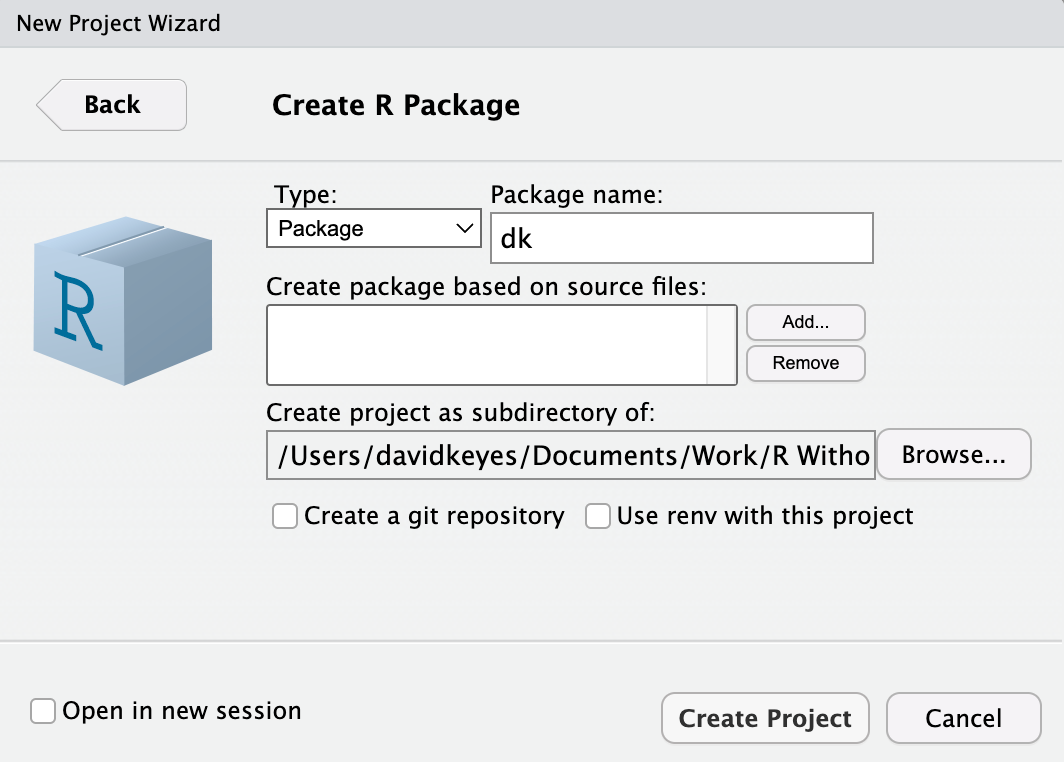
To create a package in RStudio, go to File > New Project > New Directory. Select R Package from the list of options and give your package a name. In Figure 12.2, I’ve called mine dk. Also decide where you want your package to live on your computer. You can leave everything else as is.
RStudio will now create and open the package. It should already contain a few files, including hello.R, which has a prebuilt function called hello() that, when run, prints the text Hello, world! in the console. You’ll get rid of this and a few other default files so you can start with a clean slate. Delete hello.R, NAMESPACE, and hello.Rd in the man directory.
Adding Functions with use_r()
All of the functions in a package should go in separate files in the R folder. To add these files to the package automatically and test that they work correctly, you’ll use the usethis and devtools packages. Install them using install.packages() like so:
install.packages("usethis")
install.packages("devtools")
To add a function to the package, run the use_r() function from the usethis package in the console:
usethis::use_r("acs")The package::function() syntax allows you to use a function without loading the associated package. The use_r() function should create a file in the R directory with the argument name you provide — in this case, the file is called acs.R. The name itself doesn’t really matter, but it’s a good practice to choose something that gives an indication of the functions the file contains. Now you can open the file and add code to it. Copy the get_acs_race _ethnicity() function to the package.
Checking our Package with devtools
You need to change the get_acs_race_ethnicity() function in a few ways to make it work in a package. The easiest way to figure out what changes you need to make is to use built-in tools to check that your package is built correctly. Run the function devtools::check() in the console to perform what is known as an R CMD check, a command that runs under the hood to ensure others can install your package on their system. Running R CMD check on the dk package outputs this long message:
── R CMD check results ─────────────── dk 0.1.0 ────
Duration: 4s

❯ checking DESCRIPTION meta-information ... WARNING
Non-standard license specification:
What license is it under?
Standardizable: FALSE

❯ checking for missing documentation entries ... WARNING
Undocumented code objects:
‘get_acs_race_ethnicity’
All user-level objects in a package should have documentation entries.
See chapter ‘Writing R documentation files’ in the ‘Writing R
Extensions’ manual.

❯ checking R code for possible problems ... NOTE
get_acs_race_ethnicity: no visible global function definition for
‘get_acs’
get_acs_race_ethnicity: no visible global function definition for
‘clean_names’
Undefined global functions or variables:
clean_names get_acs

0 errors ✔ | 2 warnings ✖ | 1 note ✖
The last part is the most important, so let’s review the output from bottom to top. The line 0 errors ✔ | 2 warnings ✖ | 1 note ✖ highlights three levels of issues identified in the package. Errors are the most severe, as they mean others won’t be able to install your package, while warnings and notes may cause problems for others. It’s best practice to eliminate all errors, warnings, and notes.
We’ll start by addressing the note. To help you understand what R CMD check is saying here, I need to explain a bit about how packages work. When you install a package using the install.packages() function, it often takes a while. That’s because the package you’re telling R to install likely uses functions from other packages. To access these functions, R must install these packages (known as dependencies) for you; after all, it would be a pain if you had to manually install a whole set of dependencies every time you installed a new package. But to make sure that the appropriate packages are installed for any user of the dk package, you still have to make a few changes.
R CMD check is saying this package includes several “undefined global functions or variables” and “no visible global function definition” for various functions. This is because you’re trying to use functions from the tidycensus and janitor packages, but you haven’t specified where these functions come from. I can run this code in my environment because I have tidycensus and janitor installed, but you can’t assume the same of everyone.
Adding Dependency Packages
To ensure the package’s code will work, you need to install tidycensus and janitor for users when they install the dk package. To do this, run the use_package() function from the usethis package in the console, first specifying "tidycensus" for the package argument:
usethis::use_package(package = "tidycensus")You should get the following message:
✔ Setting active project to '/Users/davidkeyes/Documents/Work/R Without Statistics/dk'
✔ Adding 'tidycensus' to Imports field in DESCRIPTION
• Refer to functions with `tidycensus::fun()`
The Setting active project... line indicates that you’re working in the dk project. The second line indicates that the DESCRIPTION file has been edited. This file provides metadata about the package you’re developing.
Next, add the janitor package the same way you added tidyverse
usethis::use_package(package = "janitor")which should give you the following output:
✔ Adding 'janitor' to Imports field in DESCRIPTION
• Refer to functions with `janitor::fun()`
If you open the DESCRIPTION file in the root directory of your project, you should see the following:
Package: dk
Type: Package
Title: What the Package Does (Title Case)
Version: 0.1.0
Author: Who wrote it
Maintainer: The package maintainer <yourself@somewhere.net>
Description: More about what it does (maybe more than one line)
    Use four spaces when indenting paragraphs within the Description.
License: What license is it under?
Encoding: UTF-8
LazyData: true
Imports:
    janitor,
    tidycensus
The Imports section at the bottom of the file indicates that when a user installs the dk package, the tidycensus and janitor packages will also be imported.
Referring to Functions Correctly
The output from running usethis::use_package(package = "janitor") also included the line Refer to functions with tidycensus::fun() (where fun() stands for function name). This tells you that in order to use functions from other packages in the dk package, you need to specify both the package name and the function name to ensure that the correct function is used at all times. On rare occasions, you’ll find functions with identical names used across multiple packages, and this syntax avoids ambiguity. Remember this line from the R CMD check?
Undefined global functions or variables:
clean_names get_acs
It appeared because you were using functions without saying what package they came from. The clean_names() function comes from the janitor package, and get_acs() comes from tidycensus, so you will need to add these package names before each function:
get_acs_race_ethnicity <- function(
  clean_variable_names = FALSE,
  ...
) {
  race_ethnicity_data <- tidycensus::get_acs(
    ...,
    variables = c(
      "White" = "B03002_003",
      "Black/African American" = "B03002_004",
      "American Indian/Alaska Native" = "B03002_005",
      "Asian" = "B03002_006",
      "Native Hawaiian/Pacific Islander" = "B03002_007",
      "Other race" = "B03002_008",
      "Multi-Race" = "B03002_009",
      "Hispanic/Latino" = "B03002_012"
    )
  )

  if (clean_variable_names == TRUE) {
    race_ethnicity_data <- janitor::clean_names(race_ethnicity_data)
  }

  race_ethnicity_data
}
Now you can run devtools::check() again, and you should see that the notes have gone away:
❯ checking DESCRIPTION meta-information ... WARNING
Non-standard license specification:
What license is it under?
Standardizable: FALSE

❯ checking for missing documentation entries ... WARNING
Undocumented code objects:
‘get_acs_race_ethnicity’
All user-level objects in a package should have documentation entries.
See chapter ‘Writing R documentation files’ in the ‘Writing R
Extensions’ manual.

0 errors ✔ | 2 warnings ✖ | 0 notes ✔
However, there are still two warnings to deal with. You’ll do that next.
Creating Documentation with Roxygen
The checking for missing documentation entries warning indicates that you need to document your get_acs_race_ethnicity() function. One of the benefits of creating a package is that you can add documentation to help others use your code. In the same way that users can enter ?get_acs() and see documentation about that function, you want them to be able to enter ?get_acs _race_ethnicity() to learn how your function works.
To create documentation for get_acs_race_ethnicity(), you’ll use Roxygen, a documentation tool that uses a package called roxygen2. To get started, place your cursor anywhere in your function. Then, in RStudio go to Code > Insert Roxygen Skeleton. This should add the following text before the get_acs_race_ethnicity() function:
#' Title
#'
#' @param clean_variable_names
#' @param ...
#'
#' @return
#' @export
#'
#' @examples
This text is the documentation’s skeleton. Each line starts with the special characters #', which indicate that you’re working with Roxygen. Now you can edit the text to create your documentation. Begin by replacing Title with a sentence that describes the function:
#' Access race and ethnicity data from the American Community SurveyNext, turn your attention to the lines beginning with @param. Roxygen automatically creates one of these lines for each function argument, but it’s up to you to fill them in with a description. Begin by describing what the clean_variable_names argument does. Next, specify that the ... will pass additional arguments to the tidycensus::get_acs() function:
#' @param clean_variable_names Should variable names be cleaned (i.e. snake case)
#' @param ... Other arguments passed to tidycensus::get_acs()
The @return line should tell the user what the get_acs_race_ethnicity() function returns. In this case, it returns data, which you document as follows:
#' @return A tibble with five variables: GEOID, NAME, variable, estimate, and moeAfter @return is @export. You don’t need to change anything here. Most functions in a package are known as exported functions, meaning they’re available to users of the package. In contrast, internal functions, which are used only by the package developers, don’t have @export in the Roxygen skeleton.
The last section is @examples. This is where you can give examples of code that users can run to learn how the function works. Doing this introduces some complexity and isn’t required, so you can skip it here and delete the line with @examples on it.
Now that you’ve added documentation with Roxygen, run devtools:: document() in the console. This should create a get_acs_race_ethnicity.Rd documentation file in the man directory using the very specific format that R packages require. You’re welcome to look at it, but you can’t change it; it’s read-only.
Running the function should also create a NAMESPACE file, which lists the functions that your package makes available to users. It should look like this:
# Generated by roxygen2: do not edit by hand

export(get_acs_race_ethnicity)
Your get_acs_race_ethnicity() function is now almost ready for users.
Adding a License and Metadata
Run devtools::check() again to see if you’ve fixed the issues that led to the warnings. The warning about missing documentation should no longer be there. However, you do still get one warning:
❯ checking DESCRIPTION meta-information ... WARNING
Non-standard license specification:
What license is it under?
Standardizable: FALSE

0 errors ✔ | 1 warning ✖ | 0 notes ✔
This warning reminds you that you have not given your package a license. If you plan to make your package publicly available, choosing a license is important because it tells other people what they can and cannot do with your code. For information about how to choose the right license for your package, see https://choosealicense.com.
In this example, you’ll use the MIT license, which allows users to do essentially whatever they want with your code, by running usethis::use_mit_license(). The usethis package has similar functions for other common licenses. You should get the following output:
✔ Setting active project to '/Users/davidkeyes/Documents/Work/R Without Statistics/dk'
✔ Setting License field in DESCRIPTION to 'MIT + file LICENSE'
✔ Writing 'LICENSE'
✔ Writing 'LICENSE.md'
✔ Adding '^LICENSE\\.md$' to '.Rbuildignore'
The use_mit_license() function handles a lot of the tedious parts of adding a license to your package. Most importantly for our purposes, it specifies the license in the DESCRIPTION file. If you open it, you should see this confirmation that you’ve added the MIT license:
License: MIT + file LICENSEIn addition to the license, the DESCRIPTION file contains metadata about the package. You can make a few changes to identify its title and add an author, a maintainer, and a description. The final DESCRIPTION file might look something like this
Package: dk
Type: Package
Title: David Keyes's Personal Package
Version: 0.1.0
Author: David Keyes
Maintainer: David Keyes <david@rfortherestofus.com>
    Description: A package with functions that David Keyes may find
    useful.
License: MIT + file LICENSE
Encoding: UTF-8
LazyData: true
Imports:
    janitor,
    tidycensus
Having made these changes, run devtools::check() one more time to make sure everything is in order:
0 errors ✔ | 0 warnings ✔ | 0 notes ✔This is exactly what you want to see!
Adding Additional Functions
You’ve now got a package with one working function in it. If you wanted to add more functions, you would follow the same procedure:
Create a new .R file with
usethis::use_r()or copy another function to the existing .R file.Develop your function using the
package::function()syntax to refer to functions from other packages.Add any dependency packages with
use_package().Add documentation for your function.
Run
devtools::check()to make sure you did everything correctly.
Your package can contain a single function, like dk, or as many functions as you want.
Installing the Package
Now you’re ready to install and use the new package. When you’re developing your own package, installing it for your own use is relatively straightforward. Simply run devtools::install(), and the package will be ready for you to use in any project.
Of course, if you’re developing a package, you’re likely doing it not just for yourself but for others as well. The most common way to make your package available to others is with the code-sharing website GitHub. The details of how to put your code on GitHub are beyond what I can cover here, but the book Happy Git and GitHub for the useR by Jenny Bryan (self-published at https://happygitwithr.com) is a great place to start.
I’ve pushed the dk package to GitHub, and you can find it at https://github.com/dgkeyes/dk. If you’d like to install it, first make sure you have the remotes package installed, then run the code remotes::install_github("dgkeyes/dk") in the console.
Summary
In this chapter, you saw that packages are useful because they let you bundle several elements needed to reliably run your code: a set of functions, instructions to automatically install dependency packages, and code documentation.
Creating your own R package is especially beneficial when you’re working for an organization, as packages can allow advanced R users to help colleagues with less experience. When Travis Gerke and Garrick Aden-Buie provided researchers at the Moffitt Cancer Center with a package that contained functions for easily accessing their databases, the researchers began to use R more creatively.
If you create a package, you can also guide people to use R in the way you think is best. Packages are a way to ensure that others follow best practices (without even being aware they are doing so). They make it easy to reuse functions across projects, help others, and adhere to a consistent style.
Additional Resources
Malcolm Barrett, “Package Development with R,” online course, accessed December 2, 2023, https://rfortherestofus.com/courses/package-development.
Hadley Wickham and Jennifer Bryan, R Packages, 2nd ed. (Sebastopol, CA: O’Reilly Media, 2023), https://r-pkgs.org.
Wrapping Up
R was invented in 1993 as a tool for statistics, and in the years since, it has been used for plenty of statistical analysis. But over the last three decades, R has also become a tool that can do much more than statistics.
As you’ve seen in this book, R is great for making visualizations. You can use it to create high-quality graphics and maps, make your own theme to keep your visuals consistent and on-brand, and generate tables that look good and communicate well. Using R Markdown or Quarto, you can create reports, presentations, and websites. And best of all, these documents are all reproducible, meaning that updating them is as easy as rerunning your code. Finally, you’ve seen that R can help you automate how you access data, as well as assist you in collaborating with others through the functions and packages you create.
If R was new to you when you started this book, I hope you now feel inspired to use it. If you’re an experienced R user, I hope this book has shown you some ways to use R that you hadn’t previously considered. No matter your background, my hope is that you now understand how to use R like a pro. Because it isn’t just a tool for statisticians — R is a tool for the rest of us too.