10 Automatically Access the Latest Data
In 2020, Meghan Harris started a job at the Primary Care Research Institute at the University of Buffalo. Her title was Data Integration Specialist, which was both generic and an accurate representation of the work she would do. One of the projects Harris worked on during her time in this job was looking at people affected by opioid use disorder, and data for this project came from a variety of surveys, all of which fed into a series of Google Sheets. She started her new job faced with a jumble of Google Sheets, tasked with helping the organization to make sense of and use its data.
For many people, especially those working in tools like SPSS, SAS, or Stata, the first step here would probably be to download the Google Sheets data. Exporting Google Sheets data to CSV or Excel files isn’t complicated so you may be wondering why I’m devoting an entire chapter to working with data from Google Sheets. Here’s why.
If R Markdown is an improvement on the typical multitool workflow discussed in Chapter 6, using the googlesheets4 package to access data directly from Google Sheets represents a similar improvement compared to downloading data each time you want to update a report. Rather than going through multiple steps (downloading data, copying it into your project, adjusting your code so it imports the new data), you can write code so that it automatically brings in new data directly from Google Sheets. Whenever you need to update your report, simply run your code and the report, generated with the latest data, will be created.
In this chapter I’ll use a simple example to demonstrate how the googlesheets4 package works. This example, using fake data on video game preferences, is one that Meghan Harris created to mirror her work with opioid survey data (which, for obvious reasons, is confidential). We’ll then conclude with some reflections on how connecting directly to data sources such as Google Sheets through R can improve your workflow.
Using the googlesheets4 Package to Bring in Up-to-Date Data
After installing the googlesheets4 package with the standard install.packages("googlesheets4"), you are ready to use it. Before you access data in a Google Sheet, you will need to connect your Google account. To do this, run the gs4_auth() function in the console. If you have more than one Google account, you will need to select the account that has access to the Google Sheet you want to work with. Once you do so, you’ll see a screen that looks like Figure 10.1.
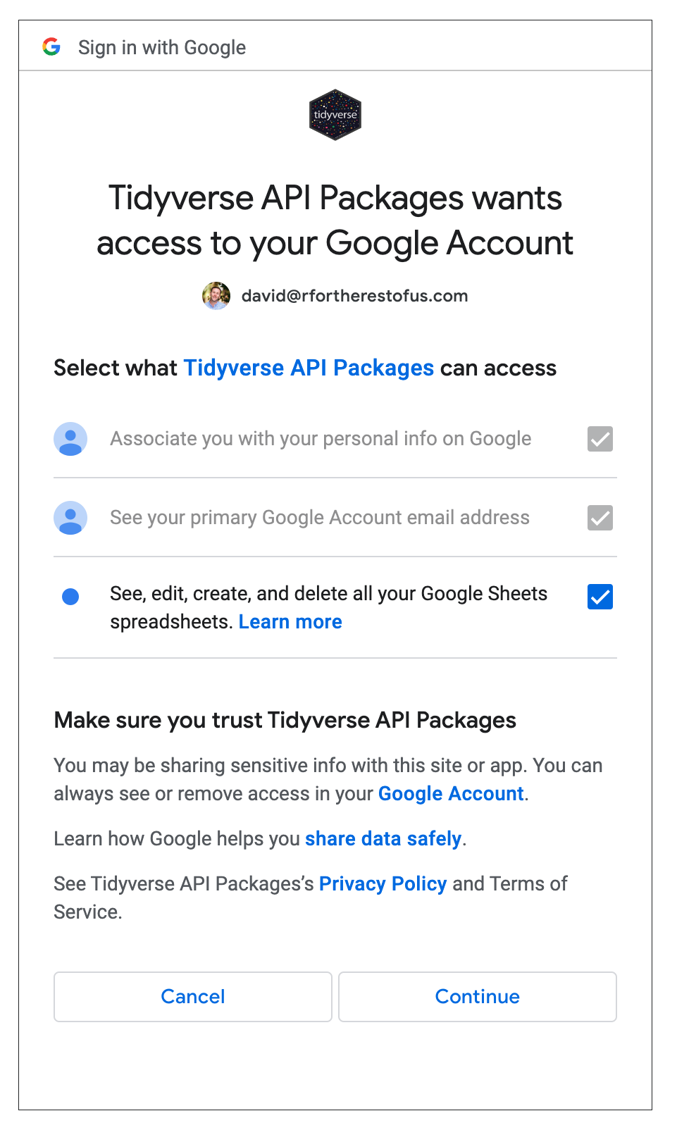
Figure 10.1: The screen asking for authorization to access your Google Sheets data
The most important thing is to check the box for “See, edit, create, and delete all your Google Sheets spreadsheets”. This will ensure that R is able to access data from your Google Sheets account. Hit Continue and you’ll be given the message “Authentication complete. Please close this page and return to R.” The googlesheets4 package will now save your credentials so that you can use them in the future without having to authenticate each time.
Now that we’ve connected R to our Google account, we can import data. We’ll import fake data that Meghan Harris created on video preferences. You can see in Figure 10.2 what it looks like in Google Sheets.
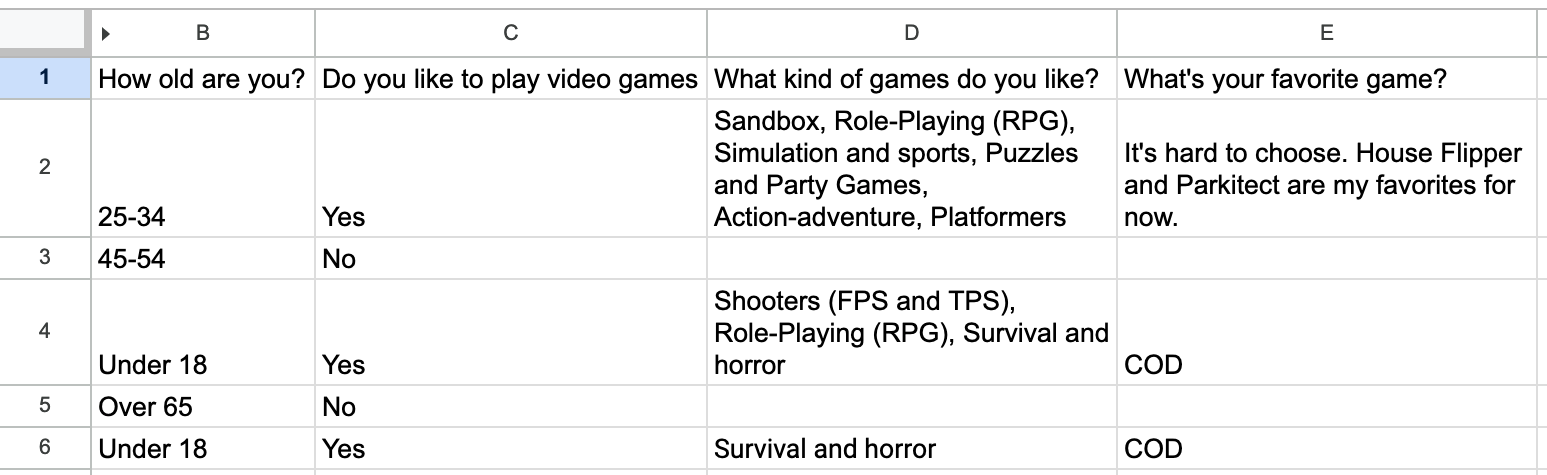
Figure 10.2: The video game data in Google Sheets
The googlesheets4 package has a function called read_sheet() that allows you to pull in data directly from a Google Sheet. We can import this data with this function in the following way:
library(googlesheets4)

survey_data_raw <- read_sheet("https://docs.google.com/spreadsheets/d/1AR0_RcFBg8wdiY4Cj-k8vRypp_txh27MyZuiRdqScog/edit?usp=sharing")
We can take a look at the survey_data_raw object to confirm that our data was imported. I’m using the glimpse() function from the dplyr package in order to make it easier to read.
The output shows that we have indeed imported the data directly from Google Sheets:
#> Rows: 5
#> Columns: 5
#> $ Timestamp                         <dttm> 2022-05-16 15:2…
#> $ `How old are you?`                <chr> "25-34", "45-54"…
#> $ `Do you like to play video games` <chr> "Yes", "No", "Ye…
#> $ `What kind of games do you like?` <chr> "Sandbox, Role-P…
#> $ `What's your favorite game?`      <chr> "It's hard to ch…
Once we have the data in R, we can now use the same workflow as always when creating reports with R Markdown. The code below is taken from an R Markdown report that Meghan Harris made to summarize the video games data. You can see the YAML, the setup code chunk, a chunk to load packages, followed by the code to read in data from Google Sheets. The next code chunk cleans the survey_data_raw object, saving the result as survey_data_clean. We then use this data to:
- Calculate the number of respondents and put this in the text using inline R code
- Create a table that shows the respondents broken down by age group
- Create a graph that shows how many respondents like video games
The code used to generate this report is below.
---
title: "Video Game Survey"
output: html_document
---

```{r setup, include=FALSE}
knitr::opts_chunk$set(echo = FALSE,
                      warning = FALSE,
                      message = FALSE)
```

```{r}
library(tidyverse)
library(janitor)
library(googlesheets4)
library(gt)
```

```{r}
# Import data from Google Sheets
survey_data_raw <- read_sheet("https://docs.google.com/spreadsheets/d/1AR0_RcFBg8wdiY4Cj-k8vRypp_txh27MyZuiRdqScog/edit?usp=sharing")
```

```{r}
# Clean data
survey_data_clean <- survey_data_raw %>%
  clean_names() %>%
  mutate("participant_id" = as.character(row_number())) %>%
  rename("age" = "how_old_are_you",
         "like_games" = "do_you_like_to_play_video_games",
         "game_types" = "what_kind_of_games_do_you_like",
         "favorite_game" = "whats_your_favorite_game") %>%
  relocate(participant_id, .before = "age") %>%
  mutate(age = factor(age, levels = c("Under 18", "18-24", "25-34", "35-44", "45-54", "55-64", "Over 65")))
```

# Respondent Demographics

```{r}
# Calculate number of respondents
number_of_respondents <- nrow(survey_data_clean)
```

We received responses from `r number_of_respondents` respondents. Their ages are below.

```{r}
survey_data_clean %>%
  select(participant_id, age) %>%
  gt() %>%
  cols_label(
    participant_id = "Participant ID",
    age = "Age"
  ) %>%
  tab_style(
    style = cell_text(weight = "bold"),
    locations = cells_column_labels()
  ) %>%
  cols_align(
    align = "left",
    columns = everything()
  ) %>%
  cols_width(
    participant_id ~ px(200),
    age ~ px(700)
  )
```

# Video Games

We asked if respondents liked video games. Their responses are below.

```{r}
survey_data_clean %>%
  count(like_games) %>%
  ggplot(aes(x = like_games,
             y = n,
             fill = like_games)) +
  geom_col() +
  scale_fill_manual(values = c(
    "No" = "#6cabdd",
    "Yes" = "#ff7400"
  )) +
  labs(title = "How Many People Like Video Games?",
       x = NULL,
       y = "Number of Participants") +
  theme_minimal(base_size = 16) +
  theme(legend.position = "none",
        panel.grid.minor = element_blank(),
        panel.grid.major.x = element_blank(),
        axis.title.y = element_blank(),
        plot.title = element_text(face = "bold",
                                  hjust = 0.5))
```
The resulting report can be seen in Figure 10.3.
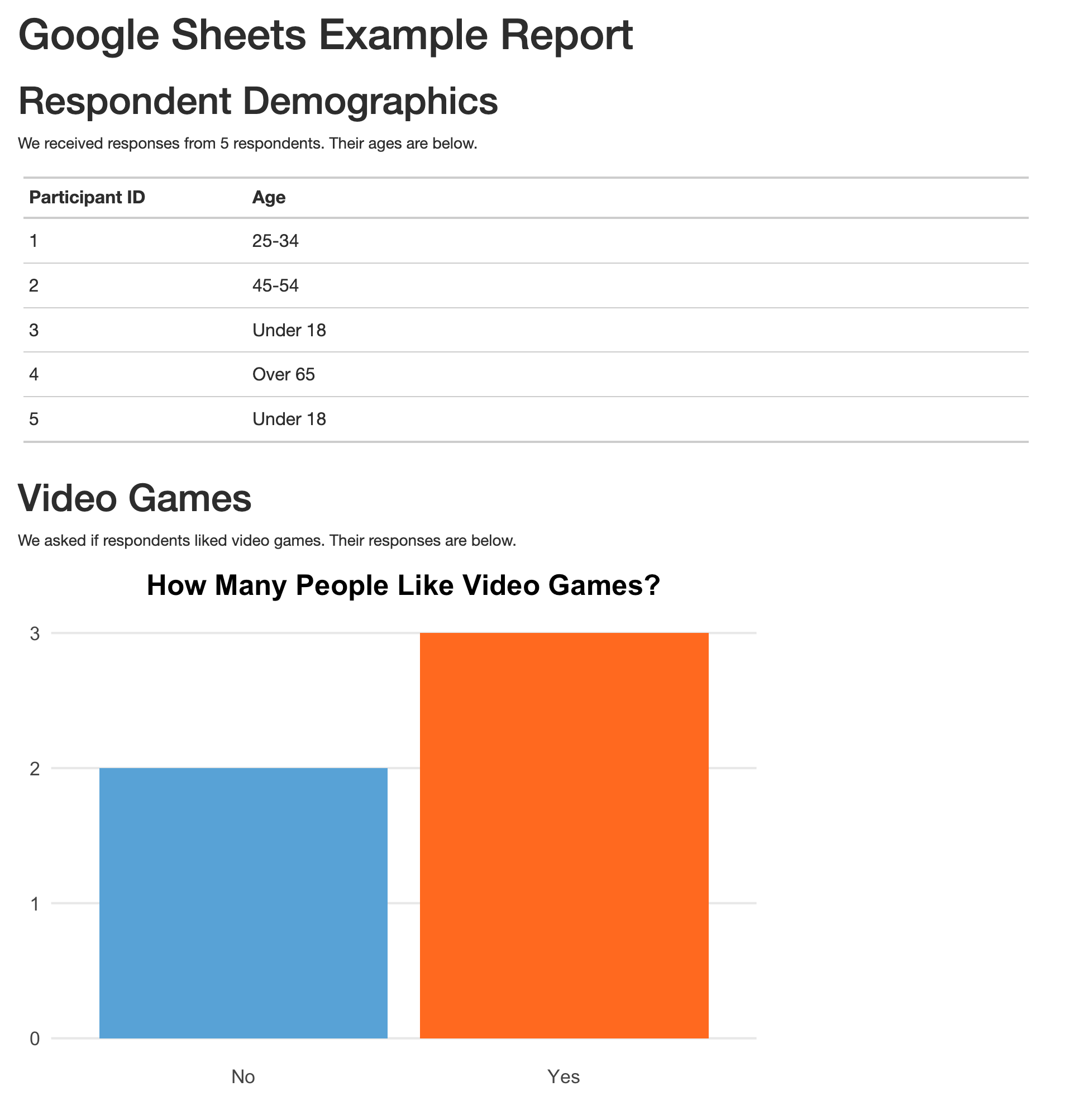
Figure 10.3: The rendered video game report
The R Markdown document here isn’t revolutionary (it’s the same types of things we saw in Chapter 6). What is different is the way we’re importing our data. Because we’re bringing it in directly from Google Sheets, there’s no risk of, say, accidentally reading in the wrong CSV. Automating this step reduces the risk of error.
The best part is that we can re-run our code at any point to bring in updated data. The read_sheet() function will look for all data on the Google Sheet we specify. Our survey had five responses today, but if we run it again tomorrow and it has additional responses, they will all be included in the import. If you use Google Forms to run your survey and have the results go to a Google Sheet, you can have an always up-to-date summary report simply by clicking the Knit button in RStudio. That workflow is one that helped Meghan Harris to collect surveys and manage a wide range of data on opiod use disorder.
Conclusion
In this chapter, we’ve shown how you can use the googlesheets4 package to import data directly from Google Sheets. This takes our reproducibility one step further, making it possible not only to generate reports automatically, but also automating the process of bringing in the latest data.
This process of bringing in data directly from the source applies beyond Google Sheets. There are packages to bring in data directly from Excel365 (Microsoft365R), Qualtrics (qualtRics), Survey Monkey (surveymonkey), and other sources. Before hitting the “Download Data” button in your data collection tool of choice, it’s worth looking into whether a package exists to import data directly into R.
For Meghan Harris, working directly with data in Google Sheets was a game-changer. She used googlesheets4 to bring in data in multiple Google Sheets. From there, she was able to streamline analysis and reporting, which ultimately had a big impact on her organization’s work. Data that had once been largely unused because accessing it was so complicated came to inform research on opioid use disorder. Bringing in data from Google Sheets with a few lines of code may seem small at first, but it can have a big impact.