---
title: "Urban Institute COVID Report"
output: html_document
params:
state: "Alabama"
---
```{r setup, include=FALSE}
knitr::opts_chunk$set(
echo = FALSE,
warning = FALSE,
message = FALSE
)
```
```{r}
library(tidyverse)
library(urbnthemes)
library(scales)
```
# `r params$state`
```{r}
cases <- tibble(state.name) %>%
rbind(state.name = "District of Columbia") %>%
left_join(
read_csv(
"united_states_covid19_cases_deaths_and_testing_by_state.csv",
skip = 2
),
by = c("state.name" = "State/Territory")
) %>%
select(
total_cases = `Total Cases`,
state.name,
cases_per_100000 = `Case Rate per 100000`
) %>%
mutate(cases_per_100000 = parse_number(cases_per_100000)) %>%
mutate(case_rank = rank(-cases_per_100000, ties.method = "min"))
```
```{r}
state_text <- if_else(params$state == "District of Columbia", str_glue("the District of Columbia"), str_glue("state of {params$state}"))
state_cases_per_100000 <- cases %>%
filter(state.name == params$state) %>%
pull(cases_per_100000) %>%
comma()
state_cases_rank <- cases %>%
filter(state.name == params$state) %>%
pull(case_rank)
```
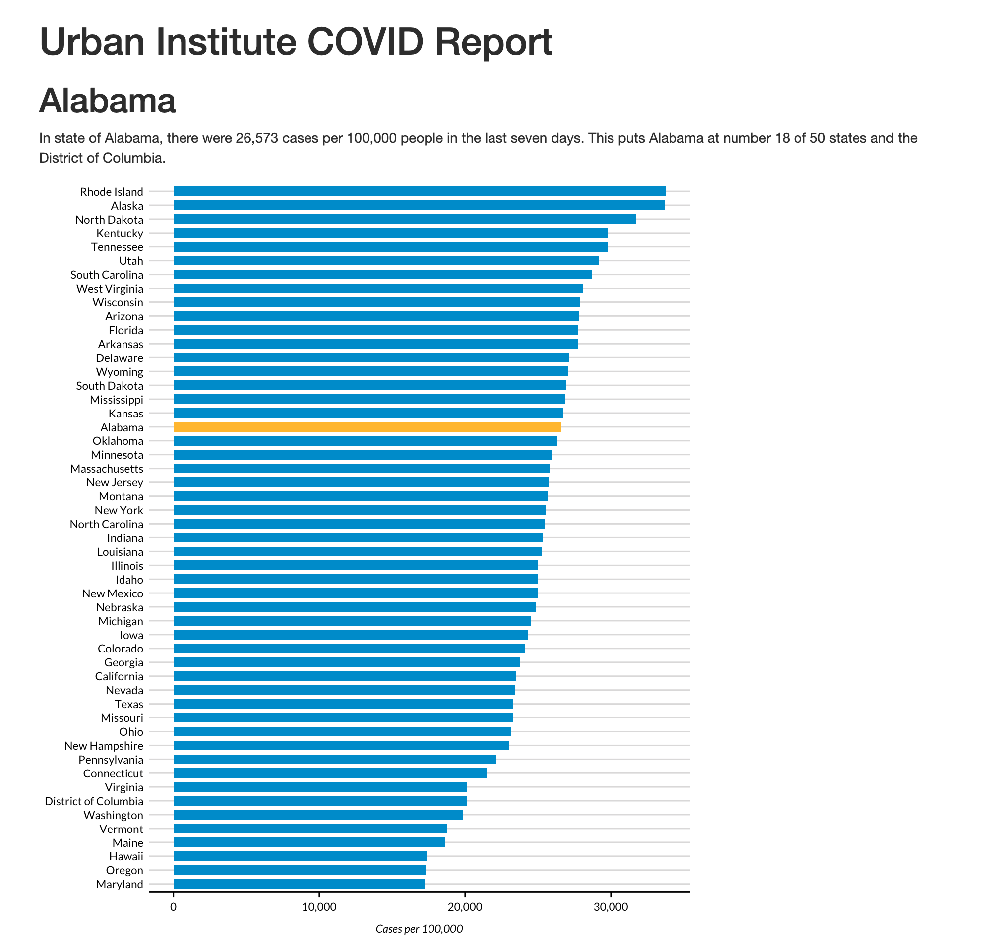
In `r state_text`, there were `r state_cases_per_100000` cases per 100,000 people in the last seven days. This puts `r params$state` at number `r state_cases_rank` of 50 states and the District of Columbia.
```{r fig.height = 8}
set_urbn_defaults(style = "print")
cases %>%
mutate(highlight_state = if_else(state.name == params$state, "Y", "N")) %>%
mutate(state.name = fct_reorder(state.name, cases_per_100000)) %>%
ggplot(aes(
x = cases_per_100000,
y = state.name,
fill = highlight_state
)) +
geom_col() +
scale_x_continuous(labels = comma_format()) +
theme(legend.position = "none") +
labs(
y = NULL,
x = "Cases per 100,000"
)
```7 Parameterized Reporting
You are reading the free online version of this book. If you’d like to purchase a physical or electronic copy, you can buy it from No Starch Press, Powell’s, Barnes and Noble or Amazon.
Parameterized reporting is a technique that allows you to generate multiple reports simultaneously. By using parameterized reporting, you can follow the same process to make 3,000 reports as you would to make one report. The technique also makes your work more accurate, as it avoids copy-and-paste errors.
Staff at the Urban Institute, a think tank based in Washington, DC, used parameterized reporting to develop fiscal briefs for all US states, as well as the District of Columbia. Each report required extensive text and multiple charts, so creating them by hand wasn’t feasible. Instead, employees Safia Sayed, Livia Mucciolo, and Aaron Williams automated the process. This chapter explains how parameterized reporting works and walks you through a simplified version of the code that the Urban Institute used.
Report Templates in R Markdown
If you’ve ever had to create multiple reports at the same time, you know how frustrating it can be, especially if you’re using the multi-tool workflow described in Chapter 6. Making just one report can take a long time. Multiply that work by 10, 20, or, in the case of the Urban Institute team, 51, and it can quickly feel overwhelming. Fortunately, with parameterized reporting, you can generate thousands of reports at once using the following workflow:
Make a report template in R Markdown.
Add a parameter (for example, one representing US states) in the YAML of your R Markdown document to represent the values that will change between reports.
Use that parameter to generate a report for one state, to make sure you can knit your document.
Create a separate R script file that sets the value of the parameter and then knits a report.
Run this script for all states.
You’ll begin by creating a report template for one state. I’ve taken the code that the Urban Institute staff used to make their state fiscal briefs and simplified it significantly. All of the packages used are ones you’ve seen in previous chapters, with the exception of the urbnthemes package. This package contains a custom ggplot theme. It can be installed by running remotes::install_github("UrbanInstitute/urbnthemes") in the console. Instead of focusing on fiscal data, I’ve used data you may be more familiar with: COVID-19 rates from mid-2022. Here’s the R Markdown document:
The text and charts in the report come from the cases data frame, shown here:
# A tibble: 51 × 4
   total_cases state.name  cases_per_100000 case_rank
   <chr>       <chr>                  <dbl>     <int>
 1 1302945     Alabama                26573        18
 2 246345      Alaska                 33675         2
 3 2025435     Arizona                27827        10
 4 837154      Arkansas               27740        12
 5 9274208     California             23472        36
 6 1388702     Colorado               24115        34
 7 766172      Connecticut            21490        43
 8 264376      Delaware               27150        13
 9 5965411     Florida                27775        11
10 2521664     Georgia                23750        35
# ℹ 41 more rows
When you knit the document, you end up with the simple HTML file shown in Figure 7.1.
You should recognize the R Markdown document’s YAML, R code chunks, inline code, and Markdown text from Chapter 6.
Defining Parameters
In R Markdown, parameters are variables that you set in the YAML to allow you to create multiple reports. Take a look at these two lines in the YAML:
params:
  state: "Alabama"
This code defines a variable called state. You can use the state variable throughout the rest of the R Markdown document with the params$variable_name syntax, replacing variable_name with state or any other name you set in the YAML. For example, consider this inline R code:
# `r params$state`Any instance of the params$state parameter will be converted to “Alabama” when you knit it. This parameter and several others appear in the following code, which sets the first-level heading visible in Figure 7.1:
In `r state_text`, there were `r state_cases_per_100000` cases per 100,000 people in the last seven days. This puts `r params$state` at number `r state_cases_rank` of 50 states and the District of Columbia. After knitting the document, you should see the following text:
In the state of Alabama, there were 26,573 cases per 100,000 people in the last seven days. This puts Alabama at number 18 of 50 states and the District of Columbia.
This text is automatically generated. The inline R code `r state_text` prints the value of the variable state_text, which is determined by a previous call to if_else(), shown in this code chunk:
state_text <- if_else(params$state == "District of Columbia", str_glue("the District of Columbia"), str_glue("state of {params$state}"))If the value of params$states is “District of Columbia”, this code sets state_text equal to “the District of Columbia”. If params$state isn’t “District of Columbia”, then state_text gets the value “state of”, followed by the state name. This allows you to put state_text in a sentence and have it work no matter whether the state parameter is a state or the District of Columbia.
Generating Numbers with Parameters
You can also use parameters to generate numeric values to include in the text. For example, to calculate the values of the state_cases_per_100000 and state_cases_rank variables dynamically, use the state parameter, as shown here:
First, this code filters the cases data frame (which contains data for all states) to keep only the data for the state in params$state. Then, the pull() function gets a single value from that data, and the comma() function from the scales package applies formatting to make state_cases_per_100000 display as 26,573 (rather than 26573). Finally, the state_cases_per_100000 and state_case_rank variables are integrated into the inline R code.
Including Parameters in Visualization Code
The params$state parameter is used in other places as well, such as to highlight a state in the report’s bar chart. To see how to accomplish this, look at the following section from the last code chunk:
cases %>%
  mutate(highlight_state = if_else(state.name == params$state, "Y", "N"))
This code creates a variable called highlight_state. Within the cases data frame, the code checks whether state.name is equal to params$state. If it is, highlight_state gets the value Y. If not, it gets N. Here’s what the relevant columns look like after you run these two lines:
# A tibble: 51 × 2
state.name highlight_state
<chr> <chr>
1 Alabama Y
2 Alaska N
3 Arizona N
4 Arkansas N
5 California N
6 Colorado N
7 Connecticut N
8 Delaware N
9 Florida N
10 Georgia N
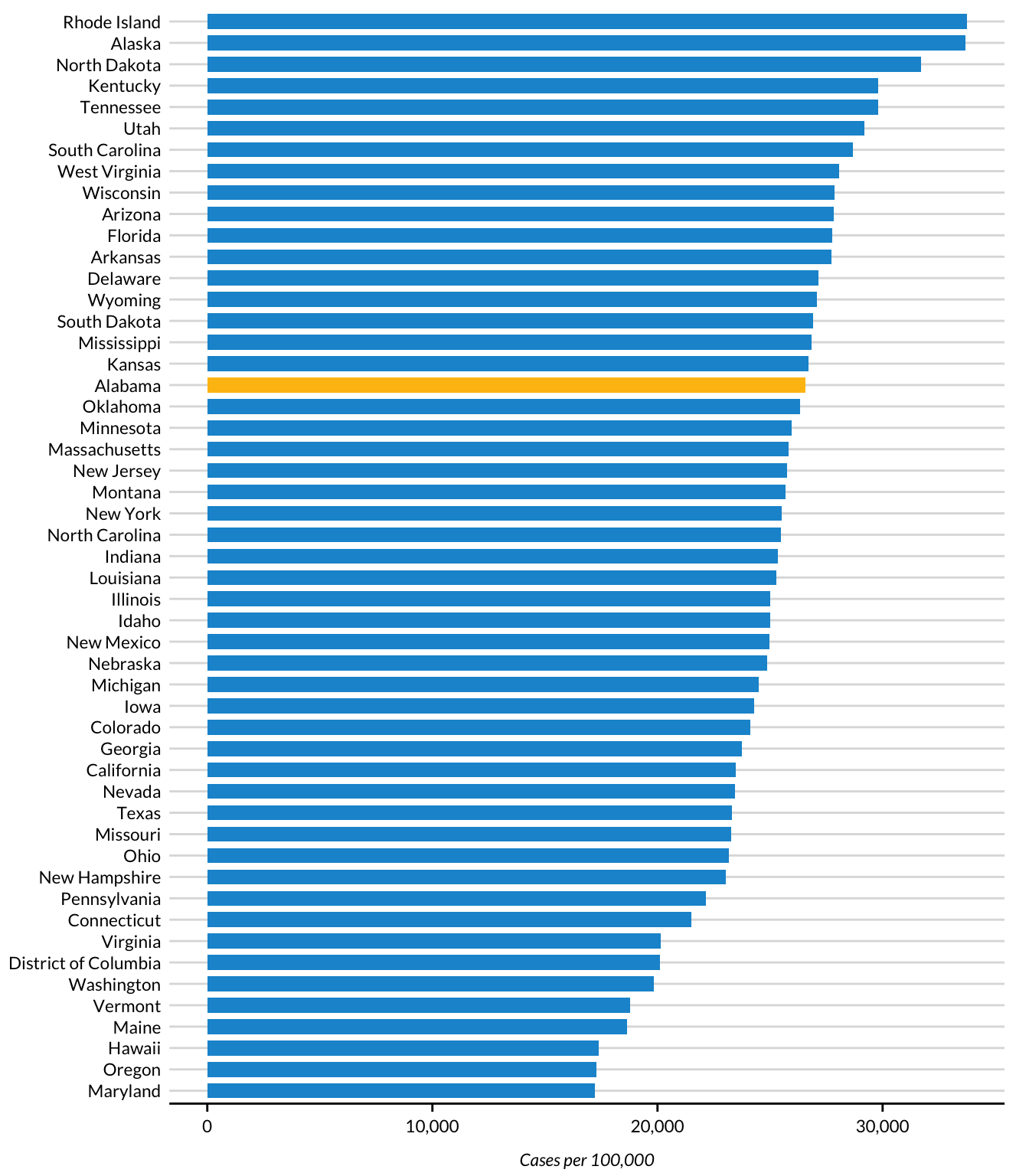
# ℹ 41 more rowsLater, the ggplot code uses the highlight_state variable for the bar chart’s fill aesthetic property, highlighting the state in params$state in yellow and coloring the other states blue. Figure 7.2 shows the chart with Alabama highlighted.
As you’ve seen, setting a parameter in the YAML allows you to dynamically generate text and charts in the knitted report. But you’ve generated only one report so far. How can you create all 51 reports? Your first thought might be to manually update the YAML by changing the parameter’s value from “Alabama” to, say, “Alaska” and then knitting the document again. While you could follow this process for all states, it would be tedious, which is what you’re trying to avoid. Instead, you can automate the report generation.
Creating an R Script
To automatically generate multiple reports based on the template you’ve created, you’ll use an R script that changes the value of the parameters in the R Markdown document and then knits it. You’ll begin by creating an R script file named render.R.
Knitting the Document with Code
Your script needs to be able to knit an R Markdown document. While you’ve seen how to do this using the Knit button, you can do the same thing with code. Load the rmarkdown package and then use its render() function as shown here:
This function generates an HTML document called urban-covid-budget-report.html. By default, the generated file has the same name as the R Markdown (.Rmd) document, with a different extension. The output_file argument assigns the file a new name, and the params argument specifies parameters that will override those in the R Markdown document itself. For example, this code tells R to use Alaska for the state parameter and save the resulting HTML file as Alaska.html.
This approach to generating reports works, but to create all 51 reports, you’d have to manually change the state name in the YAML and update the render() function before running it for each report. In the next section, you’ll update your code to make it more efficient.
Creating a Tibble with Parameter Data
To write code that generates all your reports automatically, first you must create a vector (in colloquial terms, a list of items) of all the state names and the District of Columbia. To do this, you’ll use the built-in dataset state.name, which has all 50 state names in a vector:
state <- tibble(state.name) %>%
  rbind("District of Columbia") %>%
  pull(state.name)
This code turns state.name into a tibble and then uses the rbind() function to add the District of Columbia to the list. The pull() function gets one single column and saves it as state. Here’s what the state vector looks like:
 [1] "Alabama"              "Alaska"               "Arizona"
 [4] "Arkansas"             "California"           "Colorado"
 [7] "Connecticut"          "Delaware"             "Florida"
[10] "Georgia"              "Hawaii"               "Idaho"
[13] "Illinois"             "Indiana"              "Iowa"
[16] "Kansas"               "Kentucky"             "Louisiana"
[19] "Maine"                "Maryland"             "Massachusetts"
[22] "Michigan"             "Minnesota"            "Mississippi"
[25] "Missouri"             "Montana"              "Nebraska"
[28] "Nevada"               "New Hampshire"        "New Jersey"
[31] "New Mexico"           "New York"             "North Carolina"
[34] "North Dakota"         "Ohio"                 "Oklahoma"
[37] "Oregon"               "Pennsylvania"         "Rhode Island"
[40] "South Carolina"       "South Dakota"         "Tennessee"
[43] "Texas"                "Utah"                 "Vermont"
[46] "Virginia"             "Washington"           "West Virginia"
[49] "Wisconsin"            "Wyoming"              "District of Columbia"
Rather than use render() with the input and output_file arguments, as you did earlier, you can pass it the params argument to give it parameters to use when knitting. To do so, create a tibble with the information needed to render all 51 reports and save it as an object called reports, which you’ll pass to the render() function, as follows:
reports <- tibble(
  input = "urban-covid-budget-report.Rmd",
  output_file = str_glue("{state}.html"),
  params = map(state, ~ list(state = .))
)
This code generates a tibble with 51 rows and 3 variables. In all rows, the input variable is set to the name of the R Markdown document. The value of output_file is set with str_glue() to be equal to the name of the state, followed by .html (for example, Alabama.html).
The params variable is the most complicated of the three. It is what’s known as a named list. This data structure puts the data in the state: state _name format needed for the R Markdown document’s YAML. The map() function from the purrr package creates the named list, telling R to set the value of each row as state = "Alabama", then state = "Alaska", and so on, for all of the states. You can see these variables in the reports tibble:
# A tibble: 51 × 3
   input                         output_file      params
   <chr>                         <glue>           <list>
 1 urban-covid-budget-report.Rmd Alabama.html     <named list [1]>
 2 urban-covid-budget-report.Rmd Alaska.html      <named list [1]>
 3 urban-covid-budget-report.Rmd Arizona.html     <named list [1]>
 4 urban-covid-budget-report.Rmd Arkansas.html    <named list [1]>
 5 urban-covid-budget-report.Rmd California.html  <named list [1]>
 6 urban-covid-budget-report.Rmd Colorado.html    <named list [1]>
 7 urban-covid-budget-report.Rmd Connecticut.html <named list [1]>
 8 urban-covid-budget-report.Rmd Delaware.html    <named list [1]>
 9 urban-covid-budget-report.Rmd Florida.html     <named list [1]>
10 urban-covid-budget-report.Rmd Georgia.html     <named list [1]>
# ℹ 41 more rows
The params variable shows up as <named list>, but if you open the tibble in the RStudio viewer (click reports in the Environment tab), you can see the output more clearly, as shown in Figure 7.3.
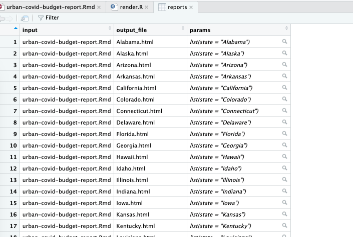
This view allows you to see the named list in the params variable, with the state variable equal to the name of each state.
Once you’ve created the reports tibble, you’re ready to render the reports. The code to do so is only one line long:
pwalk(reports, render)This pwalk() function (from the purrr package) has two arguments: a data frame or tibble (reports, in this case) and a function that runs for each row of this tibble, render().
Running this code runs the render() function for each row in reports, passing in the values for input, output_file, and params. This is equivalent to entering code like the following to run the render() function 51 times (for 50 states plus the District of Columbia):
render(
  input = "urban-covid-budget-report.Rmd",
  output_file = "Alabama.html",
  params = list(state = "Alabama")
)

render(
  input = "urban-covid-budget-report.Rmd",
  output_file = "Alaska.html",
  params = list(state = "Alaska")
)

render(
  input = "urban-covid-budget-report.Rmd",
  output_file = "Arizona.html",
  params = list(state = "Arizona")
)
Here’s the full R script file:
# Load packages
library(tidyverse)
library(rmarkdown)

# Create a vector of all states and the District of Columbia
state <- tibble(state.name) %>%
  rbind("District of Columbia") %>%
  pull(state.name)

# Create a tibble with information on the:
# input R Markdown document
# output HTML file
# parameters needed to knit the document
reports <- tibble(
  input = "urban-covid-budget-report.Rmd",
  output_file = str_glue("{state}.html"),
  params = map(state, ~ list(state = .))
)

# Generate all of our reports
pwalk(reports, render)
After running the pwalk(reports, render) code, you should see 51 HTML documents appear in the files pane in RStudio. Each document consists of a report for that state, complete with a customized graph and accompanying text.
Best Practices
While powerful, parameterized reporting can present some challenges. For example, make sure to consider outliers in your data. In the case of the state reports, Washington, DC, is an outlier because it isn’t technically a state. The Urban Institute team altered the language in the report text so that it didn’t refer to Washington, DC, as a state by using an if_else() statement, as you saw at the beginning of this chapter.
Another best practice is to manually generate and review the reports whose parameter values have the shortest (Iowa, Ohio, and Utah in the state fiscal briefs) and longest (District of Columbia) text lengths. This way, you can identify places where the text length may have unexpected results, such as cut-off chart titles or page breaks disrupted by text running onto multiple lines. A few minutes of manual review can make the process of autogenerating multiple reports much smoother.
Summary
In this chapter, you re-created the Urban Institute’s state fiscal briefs using parameterized reporting. You learned how to add a parameter to your R Markdown document, then use an R script to set the value of that parameter and knit the report.
Automating report production can be a huge time-saver, especially as the number of reports you need to generate grows. Consider another project at the Urban Institute: making county-level reports. With over 3,000 counties in the United States, creating these reports by hand isn’t realistic. Not only that, but if the Urban Institute employees were to make their reports using SPSS, Excel, and Word, they would have to copy and paste values between programs. Humans are fallible, and mistakes occur, no matter how hard we try to avoid them. Computers, on the other hand, never make copy-and-paste errors. Letting computers handle the tedious work of generating multiple reports reduces the chance of error significantly.
When you’re starting out, parameterized reporting might feel like a heavy lift, as you have to make sure that your code works for every version of your report. But once you have your R Markdown document and accompanying R script file, you should find it easy to produce multiple reports at once, saving you work in the end.
Additional Resources
Data@Urban Team, “Iterated Fact Sheets with R Markdown,” Medium, July 24, 2018, https://urban-institute.medium.com/iterated-fact-sheets-with-r-markdown-d685eb4eafce.
Data@Urban Team, “Using R Markdown to Track and Publish State Data,” Medium, April 21, 2021, https://urban-institute.medium.com/using-r-markdown-to-track-and-publish-state-data-d1291bfa1ec0.