2 - 1[1] 1R has a well-earned reputation for being hard to learn, especially for those who come to it without prior programming experience. This chapter is designed to help anyone who has never used R before. You’ll set up an R programming environment with RStudio and learn how to use functions, objects, packages, and projects to work with data. You’ll also be introduced to the tidyverse package, which contains the core data analysis and manipulation functions used in this book. This chapter won’t provide a complete introduction to R programming; rather, it will focus on the knowledge you need to follow along with the rest of the book. If you have prior experience with R, feel free to skip ahead to Chapter 2.
You’ll need two pieces of software to use R effectively. The first is R itself, which provides the underlying computational tools that make the language work. The second is an integrated development environment (IDE) like RStudio. This coding platform simplifies working with R. The best way to understand the relationship between R and RStudio is with this analogy from Chester Ismay and Albert Kim’s book Statistical Inference via Data Science: A Modern Dive into R and the Tidyverse: R is the engine that powers your data, and RStudio is like the dashboard that provides a user-friendly interface.
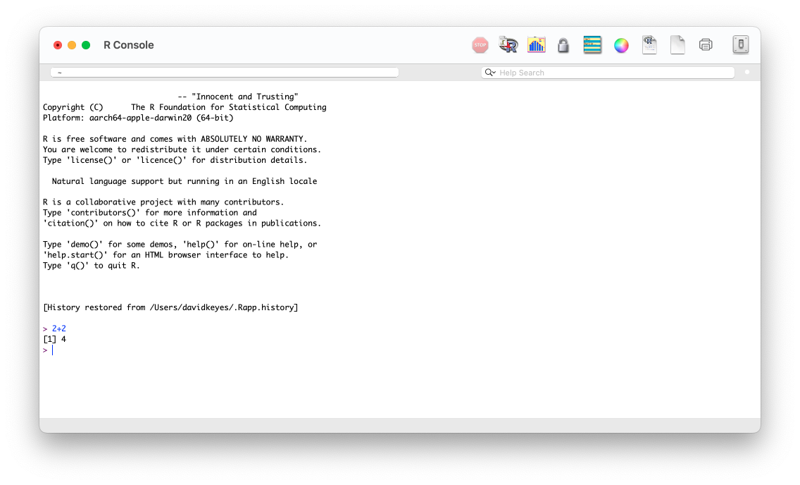
To download R, go to https://cloud.r-project.org and choose the link for your operating system. Once you’ve installed it, open the file. This should open an interface, like the one shown in Figure 1.1, that lets you work with R on your operating system’s command line. For example, enter 2 + 2, and you should see 4.
A few brave souls work with R using only this command line, but most opt to use RStudio, which provides a way to see your files, the output of your code, and more. You can download RStudio at https://posit.co/download/rstudio-desktop/. Install RStudio as you would any other app and open it.
The first time you open RStudio, you should see the three panes shown in Figure 1.2.
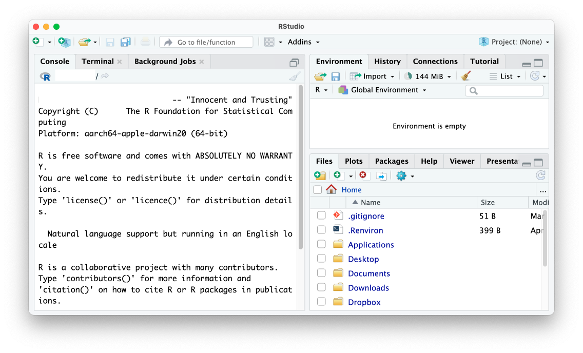
The left pane should look familiar. It’s similar to the screen you saw when working in R on the command line. This is known as the console. You’ll use it to enter code and see the results. This pane has several tabs, such as Terminal and Background Jobs, for more advanced uses. For now, you’ll stick to the default tab.
At the bottom right, the files pane shows all of the files on your computer. You can click any file to open it within RStudio. Finally, at the top right is the environment pane, which shows the objects that are available to you when working in RStudio. Objects are discussed in “Saving Data as Objects” on page 11.
There is one more pane that you’ll typically use when working in RStudio, but to see it, first you need to create an R script file.
If you write all of your code in the console, you won’t have any record of it. Say you sit down today and import your data, analyze it, and then make some graphs. If you run these operations in the console, you’ll have to re-create that code from scratch tomorrow. But if you write your code in files instead, you can run it multiple times.
R script files, which use the .R extension, save your code so you can run it later. To create an R script file, go to File > New File > R Script, and the script file pane should appear in the top left of RStudio, as shown in Figure 1.3. Save this file in your Documents folder as sample-code.R.
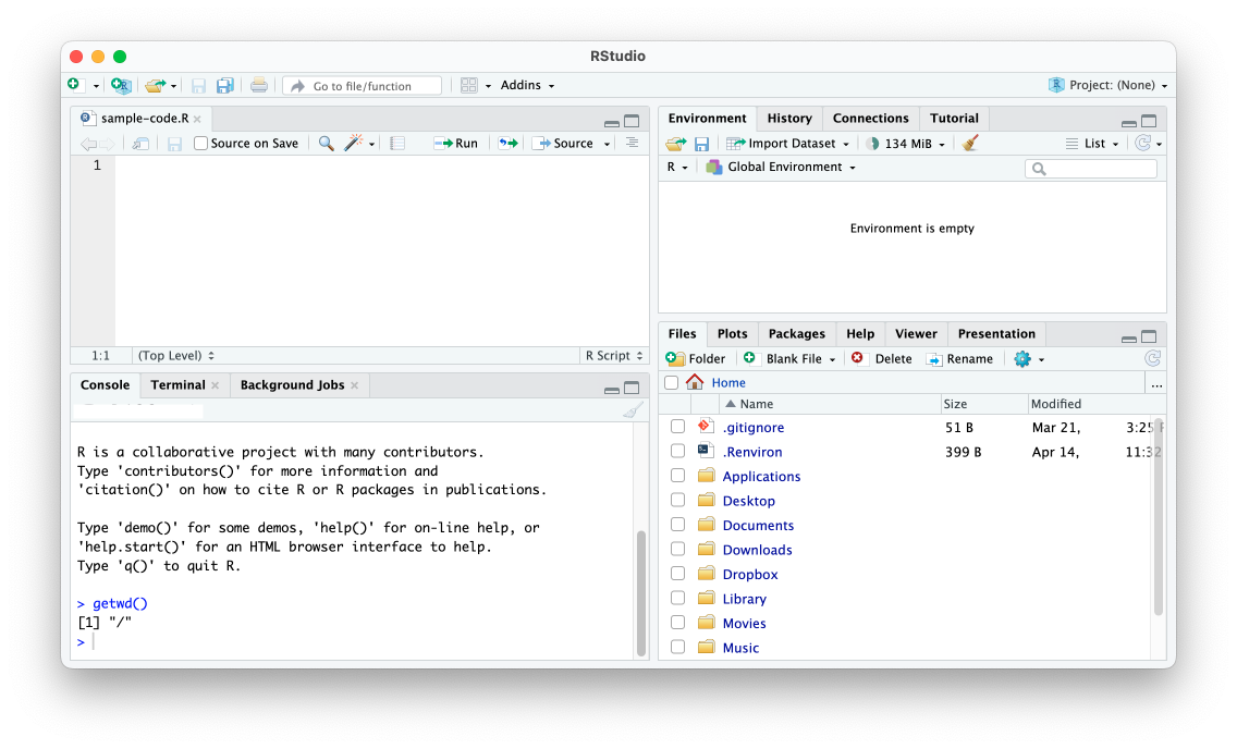
Now you can enter R code into the new pane to add it to your script file. For example, try entering 2 + 2 in the script file pane to perform a simple addition operation.
To run a script file, click Run or use the keyboard shortcut command-enter on macOS or ctrl-enter on Windows. The result (4, in this case) should show up in the console pane.
You now have a working programming environment. Next you’ll use it to write some simple R code.
If you’re trying to learn R, you probably want to perform more complex operations than 2 + 2, but understanding the fundamentals will prepare you to do more serious data analysis tasks later in this chapter. Let’s cover some of these basics.
Besides +, R supports the common arithmetic operators - for subtraction, * for multiplication, and / for division. Try entering the following in the console:
2 - 1[1] 13 * 3[1] 916 / 4[1] 4As you can see, R returns the result of each calculation you enter. You don’t have to add the spaces around operators as shown here, but doing so makes your code much more readable.
You can also use parentheses to perform multiple operations at once and see their result. The parentheses specify the order in which R will evaluate the expression. Try running the following:
2 * (2 + 1)[1] 6This code first evaluates the expression within the parentheses, 2 + 1, before multiplying the result by 2 in order to get 6.
R also has more advanced arithmetic operators, such as ** to calculate exponents:
[1] 8This is equivalent to 23, which returns 8.
To get the remainder of a division operation, you can use the %% operator:
10 %% 3[1] 1Dividing 10 by 3 produces a remainder of 1, the value R returns.
You won’t need to use these advanced arithmetic operators for the activities in this book, but they’re good to know nonetheless.
R also uses comparison operators, which let you test how one value compares to another. R will return either TRUE or FALSE. For example, enter 2 > 1 in the console:
2 > 1[1] TRUER should return TRUE, because 2 is greater than 1.
Other common comparison operators include less than (<), greater than or equal to (>=), less than or equal to (<=), equal to (==), and not equal to (!=). Here are some examples:
498 == 498[1] TRUE2 != 2[1] FALSEWhen you enter 498 == 498 in the console, R should return TRUE because the two values are equal. If you run 2 != 2 in the console, R should return FALSE because 2 does not not equal 2.
You’ll rarely use comparison operators to directly test how one value compares to another; instead, you’ll use them to perform tasks like keeping only data where a value is greater than a certain threshold. You’ll see comparison operators used in this way in “tidyverse Functions” (Section 1.6.1).
You can perform even more useful operations by making use of R’s many functions, predefined sections of code that let you efficiently do specific things. Functions have a name and a set of parentheses containing arguments, which are values that affect the function’s behavior.
Consider the print() function, which displays information:
print(x = 1.1)[1] 1.1The name of the print() function is print. Within the function’s parentheses, you specify the argument name – x, in this case — followed by the equal sign (=) and a value for the function to display. This code will print the number 1.1.
To separate multiple arguments, you use commas. For example, you can use the print() function’s digits argument to indicate how many digits of a number to display:
print(x = 1.1, digits = 1)[1] 1This code will display only one digit (in other words, a whole number).
Using these two arguments allows you to do something specific (display results) while also giving you the flexibility to change the function’s behavior.
A common R pattern is using a function within a function. For example, if you wanted to calculate the mean, or average, of the values 10, 20, and 30, you could use the mean() function to operate on the result of the c() function like so:
The c() function combines multiple values into one, which is necessary because the mean() function accepts only one argument. This is why the code has two matching sets of open and close parentheses: one for mean() and a nested one for c().
The value after the equal sign in this example, c(10, 20, 30), tells R to use the values 10, 20, and 30 to calculate the mean. Running this code in the console returns the value 20.
The functions median() and mode() work with c() in the same way. To learn how to use a function and what arguments it accepts, enter ? followed by the function’s name in the console to see the function’s help file.
Next, let’s look at how to import data for your R programs to work with.
R lets you do all of the same data manipulation tasks you might perform in a tool like Excel, such as calculating averages or totals. Conceptually, however, working with data in R is very different from working with Excel, where your data and analysis code live in the same place: a spreadsheet. While the data you work with in R might look similar to the data you work with in Excel, it typically comes from some external file, so you have to run code to import it.
You’ll import data from a comma-separated values (CSV) file, a text file that holds a series of related values separated by commas. You can open CSV files using most spreadsheet applications, which use columns rather than commas as separators. For example, Figure 1.4 shows the population-by-state.csv file in Excel.
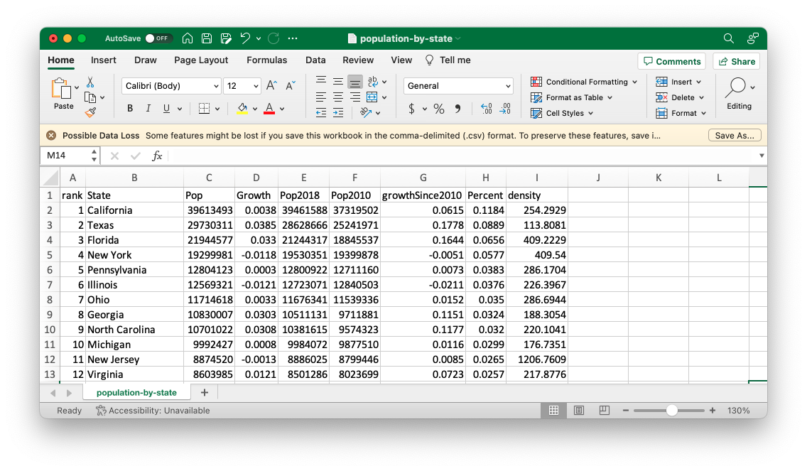
To work with this file in R, download it from https://data.rfortherestofus.com/population-by-state.csv. Save it to a location on your computer, such as your Documents folder.
Next, to import the file into R, add a line like the following to the sample-code.R file you created earlier in this chapter, replacing my filepath with the path to the file’s location on your system:
read.csv(file = "/Users/davidkeyes/Documents/population-by-state.csv")The file argument in the read.csv() function specifies the path to the file to open.
The read.csv() function can accept additional optional arguments, separated by commas. For example, the following line uses the skip argument in addition to file to import the same file but skip the first row:
read.csv(
  file = "/Users/davidkeyes/Documents/population-by-state.csv",
  skip = 1
)
To learn about additional arguments for this function, enter ?read.csv() in the console to see its help file.
At this point, you can run the code to import your data (without the skip argument). Highlight the line you want to run in the script file pane in RStudio and click Run. You should see the following output in the console pane:
   rank                State      Pop  Growth  Pop2018  Pop2010 growthSince2010
1     1           California 39613493  0.0038 39461588 37319502          0.0615
2     2                Texas 29730311  0.0385 28628666 25241971          0.1778
3     3              Florida 21944577  0.0330 21244317 18845537          0.1644
4     4             New York 19299981 -0.0118 19530351 19399878         -0.0051
5     5         Pennsylvania 12804123  0.0003 12800922 12711160          0.0073
6     6             Illinois 12569321 -0.0121 12723071 12840503         -0.0211
7     7                 Ohio 11714618  0.0033 11676341 11539336          0.0152
8     8              Georgia 10830007  0.0303 10511131  9711881          0.1151
9     9       North Carolina 10701022  0.0308 10381615  9574323          0.1177
10   10             Michigan  9992427  0.0008  9984072  9877510          0.0116
11   11           New Jersey  8874520 -0.0013  8886025  8799446          0.0085
12   12             Virginia  8603985  0.0121  8501286  8023699          0.0723
13   13           Washington  7796941  0.0363  7523869  6742830          0.1563
14   14              Arizona  7520103  0.0506  7158024  6407172          0.1737
15   15            Tennessee  6944260  0.0255  6771631  6355311          0.0927
16   16        Massachusetts  6912239  0.0043  6882635  6566307          0.0527
17   17              Indiana  6805663  0.0165  6695497  6490432          0.0486
18   18             Missouri  6169038  0.0077  6121623  5995974          0.0289
19   19             Maryland  6065436  0.0049  6035802  5788645          0.0478
20   20             Colorado  5893634  0.0356  5691287  5047349          0.1677
21   21            Wisconsin  5852490  0.0078  5807406  5690475          0.0285
22   22            Minnesota  5706398  0.0179  5606249  5310828          0.0745
23   23       South Carolina  5277830  0.0381  5084156  4635649          0.1385
24   24              Alabama  4934193  0.0095  4887681  4785437          0.0311
25   25            Louisiana  4627002 -0.0070  4659690  4544532          0.0181
26   26             Kentucky  4480713  0.0044  4461153  4348181          0.0305
27   27               Oregon  4289439  0.0257  4181886  3837491          0.1178
28   28             Oklahoma  3990443  0.0127  3940235  3759944          0.0613
29   29          Connecticut  3552821 -0.0052  3571520  3579114         -0.0073
30   30                 Utah  3310774  0.0499  3153550  2775332          0.1929
31   31          Puerto Rico  3194374  0.0003  3193354  3721525         -0.1416
32   32               Nevada  3185786  0.0523  3027341  2702405          0.1789
33   33                 Iowa  3167974  0.0061  3148618  3050745          0.0384
34   34             Arkansas  3033946  0.0080  3009733  2921964          0.0383
35   35          Mississippi  2966407 -0.0049  2981020  2970548         -0.0014
36   36               Kansas  2917224  0.0020  2911359  2858190          0.0207
37   37           New Mexico  2105005  0.0059  2092741  2064552          0.0196
38   38             Nebraska  1951996  0.0137  1925614  1829542          0.0669
39   39                Idaho  1860123  0.0626  1750536  1570746          0.1842
40   40        West Virginia  1767859 -0.0202  1804291  1854239         -0.0466
41   41               Hawaii  1406430 -0.0100  1420593  1363963          0.0311
42   42        New Hampshire  1372203  0.0138  1353465  1316762          0.0421
43   43                Maine  1354522  0.0115  1339057  1327629          0.0203
44   44              Montana  1085004  0.0229  1060665   990697          0.0952
45   45         Rhode Island  1061509  0.0030  1058287  1053959          0.0072
46   46             Delaware   990334  0.0257   965479   899593          0.1009
47   47         South Dakota   896581  0.0204   878698   816166          0.0985
48   48         North Dakota   770026  0.0158   758080   674715          0.1413
49   49               Alaska   724357 -0.0147   735139   713910          0.0146
50   50 District of Columbia   714153  0.0180   701547   605226          0.1800
51   51              Vermont   623251 -0.0018   624358   625879         -0.0042
52   52              Wyoming   581075  0.0060   577601   564487          0.0294
   Percent    density
1   0.1184   254.2929
2   0.0889   113.8081
3   0.0656   409.2229
4   0.0577   409.5400
5   0.0383   286.1704
6   0.0376   226.3967
7   0.0350   286.6944
8   0.0324   188.3054
9   0.0320   220.1041
10  0.0299   176.7351
11  0.0265  1206.7609
12  0.0257   217.8776
13  0.0233   117.3249
14  0.0225    66.2016
15  0.0208   168.4069
16  0.0207   886.1845
17  0.0203   189.9644
18  0.0184    89.7419
19  0.0181   624.8518
20  0.0176    56.8653
21  0.0175   108.0633
22  0.0171    71.6641
23  0.0158   175.5707
24  0.0147    97.4271
25  0.0138   107.0966
26  0.0134   113.4760
27  0.0128    44.6872
28  0.0119    58.1740
29  0.0106   733.7507
30  0.0099    40.2918
31  0.0095   923.4964
32  0.0095    29.0195
33  0.0095    56.7158
34  0.0091    58.3059
35  0.0089    63.2186
36  0.0087    35.6808
37  0.0063    17.3540
38  0.0058    25.4087
39  0.0056    22.5079
40  0.0053    73.5443
41  0.0042   218.9678
42  0.0041   153.2674
43  0.0040    43.9167
44  0.0032     7.4547
45  0.0032  1026.6044
46  0.0030   508.1242
47  0.0027    11.8265
48  0.0023    11.1596
49  0.0022     1.2694
50  0.0021 11707.4262
51  0.0019    67.6197
52  0.0017     5.9847
This is R’s way of confirming that it imported the CSV file and understands the data within it. Four variables show each state’s rank (in terms of population size), name, current population, population growth between the Pop and Pop2018 variables (expressed as a percentage), and 2018 population. Several other variables are hidden in the output, but you’ll see them if you import this CSV file yourself.
You might think you’re ready to work with your data now, but all you’ve really done at this point is display the result of running the code that imports the data. To actually use the data, you need to save it to an object.
To save your data for reuse, you need to create an object. For the purposes of this discussion, an object is a data structure that is stored for later use. To create an object, update your data-importing syntax so it looks like this:
Now this line of code contains the <- assignment operator, which takes what follows it and assigns it to the item on the left. To the left of the assignment operator is the population_data object. Put together, the whole line imports the CSV file and assigns it to an object called population_data.
When you run this code, you should see population_data in your environment pane, as shown in Figure 1.5.
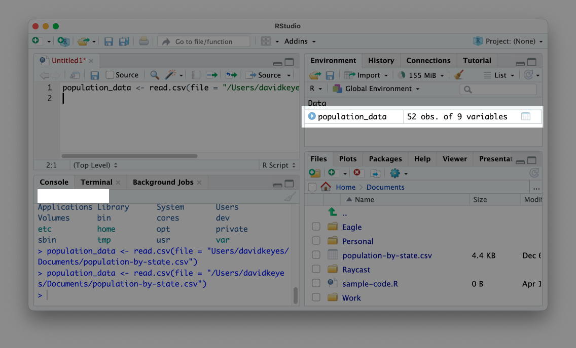
This message confirms that your data import worked and that the population_data object is ready for future use. Now, instead of having to rerun the code to import the data, you can simply enter population_data in an R script file or in the console to output the data.
Data imported to an object in this way is known as a data frame. You can see that the population_data data frame has 52 observations and 9 variables. Variables are the data frame’s columns, each of which represents some value (for example, the population of each state). As you’ll see throughout the book, you can add new variables or modify existing ones using R code. The 52 observations come from the 50 states, as well as the District of Columbia and Puerto Rico.
population_data <- read.csv(file = "/Users/davidkeyes/Documents/population-by-state.csv")The read.csv() function you’ve been using, as well as the mean() and c() functions you saw earlier, comes from base R, the set of built-in R functions. To use base R functions, you simply enter their names. However, one of the benefits of R being an open source language is that anyone can create their own code and share it with others. R users around the world make R packages, which provide custom functions to accomplish specific goals.
The best analogy for understanding packages also comes from the book Statistical Inference via Data Science. The functionality in base R is like the features built into a smartphone. A smartphone can do a lot on its own, but you usually want to install additional apps for specific tasks. Packages are like apps, giving you functionality beyond what’s built into base R. In Chapter 12, you’ll create your own R package.
You can install packages using the install.packages() function. You’ll be working with the tidyverse package, which provides a range of functions for data import, cleaning, analysis, visualization, and more. To install it, enter install.packages("tidyverse"). Typically, you’ll enter package installation code in the console rather than in a script file because you need to install a package only once on your computer to access its code in the future.
To confirm that the tidyverse package has been installed correctly, click the Packages tab on the bottom-right pane in RStudio. Search for tidyverse, and you should see it pop up.
Now that you’ve installed the tidyverse, you’ll put it to use. Although you need to install packages only once per computer, you need to load them each time you restart RStudio. Return to the sample-code.R file and reimport your data using a function from the tidyverse package (your filepath will look slightly different):
At the top of the script, the line library(tidyverse) loads the tidyverse package. Then, the package’s read_csv() function imports the data. Note the underscore (_) in place of the period (.) in the function’s name; this differs from the base R function you used earlier. Using read_csv() to import CSV files achieves the same goal of creating an object, however — in this case, one called population_data_2. Enter population_data_2 in the console, and you should see this output:
population_data_2 <- read_csv(file = "data/population-by-state.csv")

population_data_2
# A tibble: 52 × 9
rank State Pop Growth Pop2018 Pop2010 growthSince2010 Percent density
<dbl> <chr> <dbl> <dbl> <dbl> <dbl> <dbl> <dbl> <dbl>
1 1 Califor… 3.96e7 0.0038 3.95e7 3.73e7 0.0615 0.118 254.
2 2 Texas 2.97e7 0.0385 2.86e7 2.52e7 0.178 0.0889 114.
3 3 Florida 2.19e7 0.033 2.12e7 1.88e7 0.164 0.0656 409.
4 4 New York 1.93e7 -0.0118 1.95e7 1.94e7 -0.0051 0.0577 410.
5 5 Pennsyl… 1.28e7 0.0003 1.28e7 1.27e7 0.0073 0.0383 286.
6 6 Illinois 1.26e7 -0.0121 1.27e7 1.28e7 -0.0211 0.0376 226.
7 7 Ohio 1.17e7 0.0033 1.17e7 1.15e7 0.0152 0.035 287.
8 8 Georgia 1.08e7 0.0303 1.05e7 9.71e6 0.115 0.0324 188.
9 9 North C… 1.07e7 0.0308 1.04e7 9.57e6 0.118 0.032 220.
10 10 Michigan 9.99e6 0.0008 9.98e6 9.88e6 0.0116 0.0299 177.
# ℹ 42 more rowsThis data looks slightly different from the data you generated using the read.csv() function. For example, R shows only the first 10 rows. This variation occurs because read_csv() imports the data not as a data frame but as a data type called a tibble. Both data frames and tibbles are used to describe rectangular data like what you would see in a spreadsheet. There are some minor differences between data frames and tibbles, the most important of which is that tibbles print only the first 10 rows by default, while data frames print all rows. For the purposes of this book, the two terms are used interchangeably.
So far, you’ve imported a CSV file from your Documents folder. But because others won’t have this exact location on their computer, your code won’t work if they try to run it. One solution to this problem is an RStudio project.
By working in a project, you can use relative paths to your files instead of having to write the entire filepath when calling a function to import data. Then, if you place the CSV file in your project, anyone can open it by using the file’s name, as in read_csv(file = "population-by-state.csv"). This makes the path easier to write and enables others to use your code.
To create a new RStudio project, go to File New Project. Select either New Directory or Existing Directory and choose where to put your project. If you choose New Directory, you’ll need to specify that you want to create a new project. Next, choose a name for the new directory and where it should live. (Leave the checkboxes that ask about creating a Git repository and using renv unchecked; they’re for more advanced purposes.)
Once you’ve created this project, you should see two major differences in RStudio’s appearance. First, the files pane no longer shows every file on your computer. Instead, it shows only files in the example-project directory. Right now, that’s just the example-project.Rproj file, which indicates that the folder contains a project. Second, at the top right of RStudio, you can see the name example-project. This label previously read Project: (None). If you want to make sure you’re working in a project, check for its name here. Figure 1.6 shows these changes.
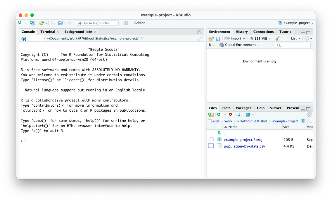
Now that you’ve created a project, copy the population-by-state.csv file into the example-project directory. Once you’ve done so, you should see it in the RStudio files pane.
With this CSV file in your project, you can now import it more easily. As before, start by loading the tidyverse package. Then, remove the reference to the Documents folder and import your data by simply using the name of the file:
The reason you can import the population-by-state.csv file this way is that the RStudio project sets the working directory to be the root of your project. With the working directory set like this, all references to files are relative to the .Rproj file at the root of the project. Now anyone can run this code because it imports the data from a location that is guaranteed to exist on their computer.
Now that you’ve imported the population data, you’re ready to do a bit of analysis on it. Although I’ve been referring to the tidyverse as a single package, it’s actually a collection of packages. We’ll explore several of its functions throughout this book, but this section introduces you to its basic workflow.
Because you’ve loaded the tidyverse package, you can now access its functions. For example, the package’s summarize() function takes a data frame or tibble and calculates some piece of information for one or more of the variables in that dataset. The following code uses summarize() to calculate the mean population of all states:
First, the code passes population_data_2 to the summarize() function’s .data argument to tell R to use that data frame to perform the calculation. Next, it creates a new variable called mean_population and assigns it to the output of the mean() function introduced earlier. The mean() function runs on Pop, one of the variables in the population_data_2 data frame.
You might be wondering why you don’t need to use the c() function within mean(), as shown earlier in this chapter. The reason is that you’re passing the function only one argument here: Pop, which contains the set of population data for which you’re calculating the mean. In this case, there’s no need to use c() to combine multiple values into one.
Running this code should return a tibble with a single variable (mean_population), as shown here:
# A tibble: 1 × 1
  mean_population
            <dbl>
1        6433422.
The variable is of type double (dbl), which is used to hold general numeric data. Other common data types are integer (for whole numbers, such as 4, 82, and 915), character (for text values), and logical (for the TRUE/FALSE values returned from comparison operations). The mean_population variable has a value of 6433422, the mean population of all states.
Notice also that the summarize() function creates a totally new tibble from the original population_data_2 data frame. This is why the variables from population_data_2 are no longer present in the output. This is a basic example of data analysis, but you can do a lot more with the tidyverse.
One advantage of working with the tidyverse is that it uses the pipe for multi-step operations. The tidyverse pipe, which is written as %>%, allows you to break steps into multiple lines. For example, you could rewrite your code using the pipe like so:
This code says, “Start with the population_data_2 data frame, then run the summarize() function on it, creating a variable called mean_population by calculating the mean of the Pop variable.”
Notice that the line following the pipe is indented. To make the code easier to read, RStudio automatically adds two spaces to the start of lines that follow pipes.
The pipe becomes even more useful when you use multiple steps in your data analysis. Say, for example, you want to calculate the mean population of the five largest states. The following code adds a line that uses the filter() function, also from the tidyverse package, to include only states where the rank variable is less than or equal to (<=) 5. Then, it uses summarize() to calculate the mean of those states:
Running this code returns the mean population of the five largest states:
# A tibble: 1 × 1
  mean_population
            <dbl>
1        24678497
Using the pipe to combine functions lets you refine your data in multiple ways while keeping it readable and easy to understand. Indentation can also make your code more readable. You’ve seen only a few functions for analysis at this point, but the tidyverse has many more functions that enable you to do nearly anything you could hope to do with your data. Because of how useful the tidyverse is, it will appear in every single piece of R code you write in this book.
Now that you’ve learned the basics of how R works, you’re probably ready to dive in and write some code. When you do, though, you’re going to encounter errors. Being able to get help when you run into issues is a key part of learning to use R successfully. There are two main strategies you can use to get unstuck.
The first is to read the documentation for the functions you use. Remember, to access the documentation for any function, simply enter ? and then the name of the function in the console. In the bottom-right pane in Figure 1.7, for example, you can see the result of running ?read.csv.
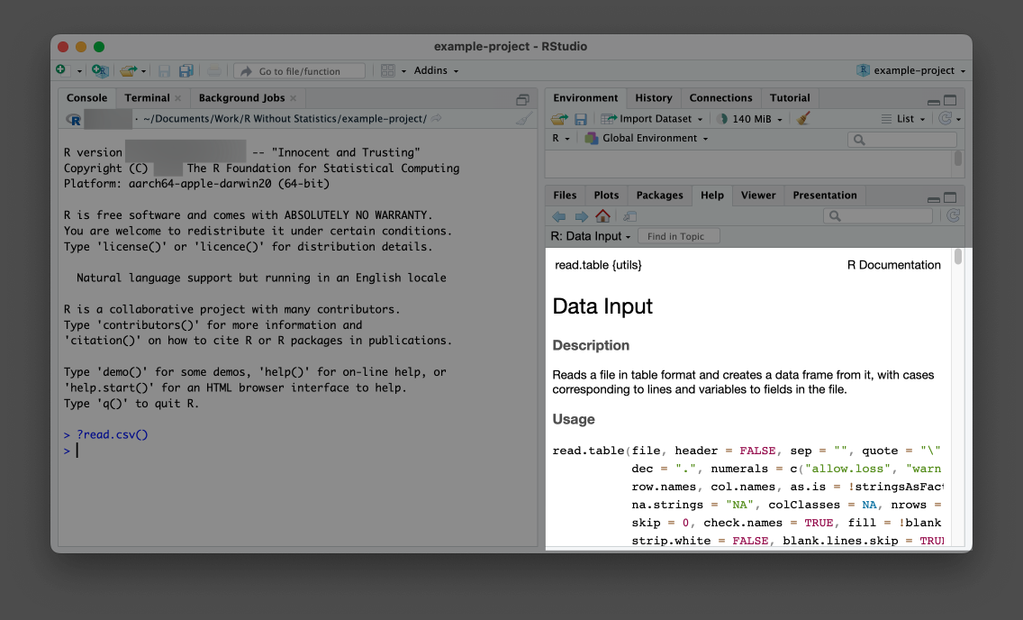
read.csv() function
Help files can be a bit hard to decipher, but essentially they describe what package the function comes from, what the function does, what arguments it accepts, and some examples of how to use it.
The second approach is to read the documentation websites associated with many R packages. These can be easier to read than RStudio’s help files. In addition, they often contain longer articles, known as vignettes, that provide an overview of how a given package works. Reading these can help you understand how to combine individual functions in the context of a larger project. Every package discussed in this book has a good documentation website.
In this chapter, you learned the basics of R programming. You saw how to download and set up R and RStudio, what the various RStudio panes are for, and how R script files work. You also learned how to import CSV files and explore them in R, how to save data as objects, and how to install packages to access additional functions. Then, to make the files used in your code more accessible, you created an RStudio project. Finally, you experimented with tidyverse functions and the tidyverse pipe, and you learned how to get help when those functions don’t work as expected.
Now that you understand the basics, you’re ready to start using R to work with your data. See you in Chapter 2!
Comments
In addition to code, R script files often contain comments — lines that begin with hash marks (
#) and aren’t treated as runnable code but instead as notes for anyone reading the script. For example, you could add a comment to the code from the previous section, like so:This comment will help others understand what is happening in the code, and it can also serve as a useful reminder for you if you haven’t worked on the code in a while. R knows to ignore any lines that begin with the hash mark instead of trying to run them.